Asynchronous Advantage Actor Critic (A3C)

We have discussed the details of the Vanilla Actor-Critic (VAC) and implemented an application for stock prediction. Today, I would like to explore another variation of the Actor-Critic family called Asynchronous Advantage Actor-Critic (A3C), which is the predecessor of Actor-Critic (A2C). Actor Critic (A2C).

In brief, A3C is basically vanilla actor-critic enhanced with parallel asynchronous workers to make training faster and stable.

Formal Definition of A3C

Here, I only define the core elements of this algorithm; you can refer to other concepts in the following post. The main differences compared to VAC are the use of the advantage function and entropy regularization. The following illustrates the mechanism of this algorithm.

Vanilla Actor-Critic (VAC)

We have previously discussed the Actor Critic and Soft Actor Critic (SAC) frameworks. Today, I would like to revisit its most fundamental form in order to build a deeper understanding and connect it to real-world applications. Specifically, I will focus on the Vanilla Actor–Critic (VAC) algorithm, explaining its details

CSYYYSCCSY

Components

1. Actor and Critic (Policy/Value Network)

$$π_\theta(a|s) = P(A_t = a | S_t = s), \quad V_{\phi}(s) \approx 𝔼[R_t|S_t = s]$$

2. Advantage Function: measures relative goodness of an action

$$A_t = G_t - V_{\phi}(s_t), \quad R_t = \sum_{k=0}^{n-1} \gamma^k r_{t+k} + \gamma^n V_{\phi}(s_{t+n})$$

3. Entropy Regularization: encourages exploration

$$L_{entropy}(\theta) = -\sum_{a}π_{\theta}(a|s_t)\log π_{\theta}(a|s_t)$$

Update Rules

Here shows the rules simply.

1. Policy and Value Loss (Actor/Critic Network)

$$L_{\text{policy}}(\theta) = -\log π_{\theta}(a_t|s_t) \cdot A_t, \quad L_{\text{value}}(\phi) = (R_t - V_{\phi}(s_t))^2$$

2. Total Loss

$$J(\theta, \phi) = L_{\text{total}}(\theta, \phi) = L_{\text{policy}}(\theta) - c_1 \cdot L_{\text{value}}(\phi) + c_2 \cdot L_{\text{entropy}}(\theta)$$

3. Networks Update

$$\theta \leftarrow \theta + \alpha_1 \nabla_{\theta}J(\theta, \phi)$$

$$\phi \leftarrow \phi + \alpha_2 \nabla_{\phi}J(\theta, \phi)$$

Real-World Application - Stock Prediction

We add new agent to the same project created at Vanilla Actor-Critic (VAC). The A3C agent should train faster, and stable than VAC. The features and training configuration are the same to VAC. Let's also experiment this agent on NVDA and SOFI as our targets. Let's see how it works.

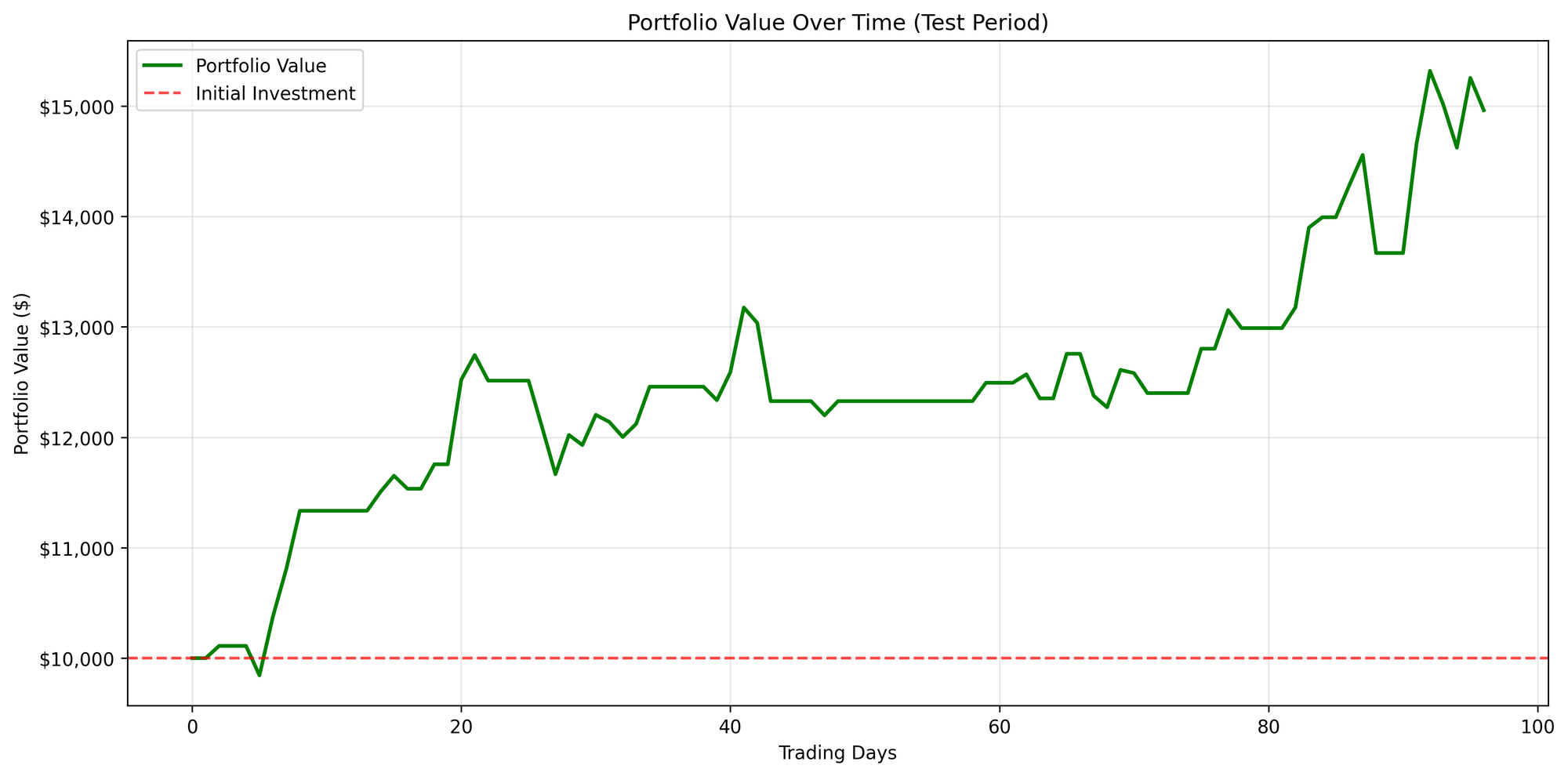
Figure A: SOFI

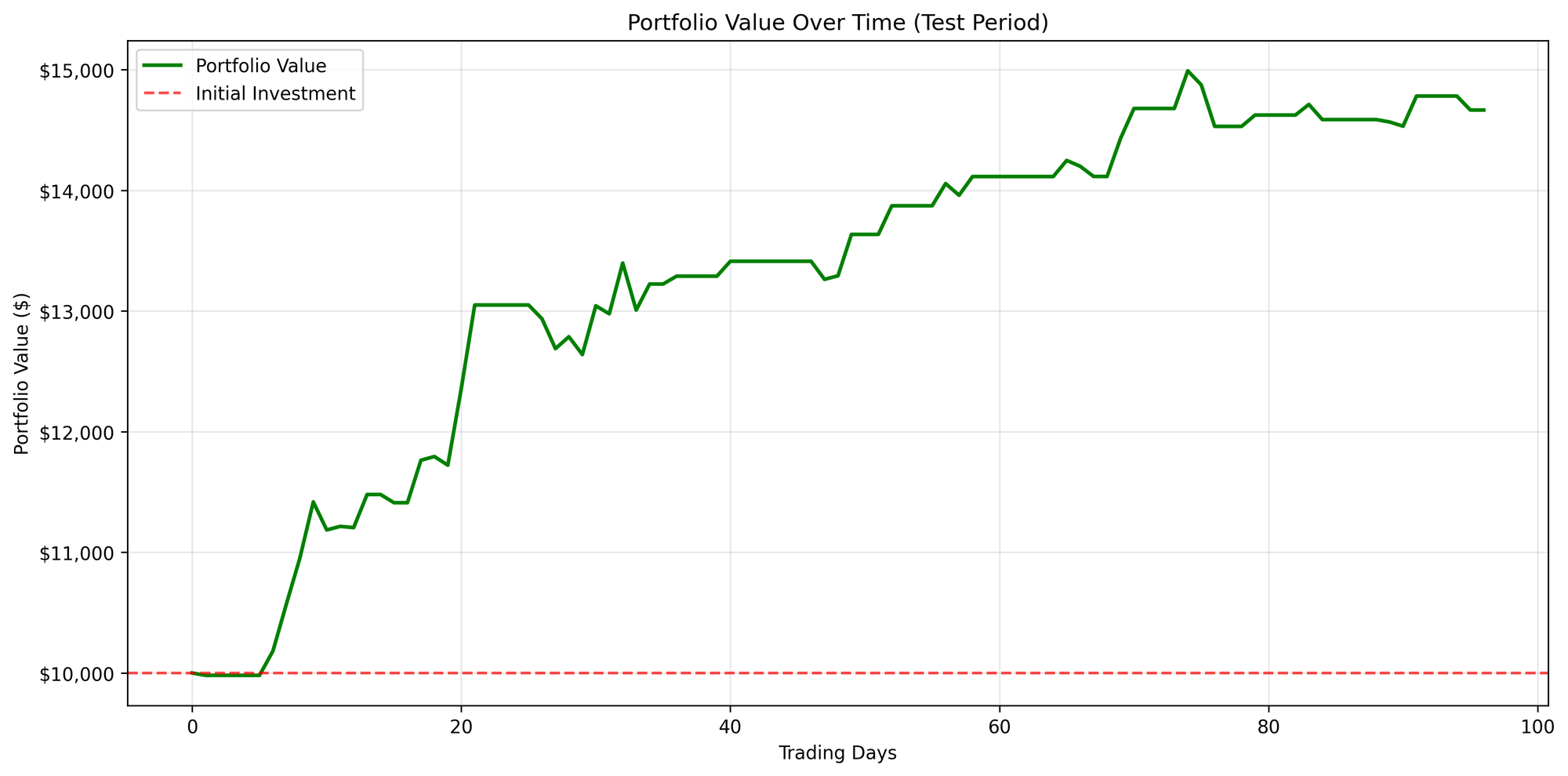
Figure B: NVDA

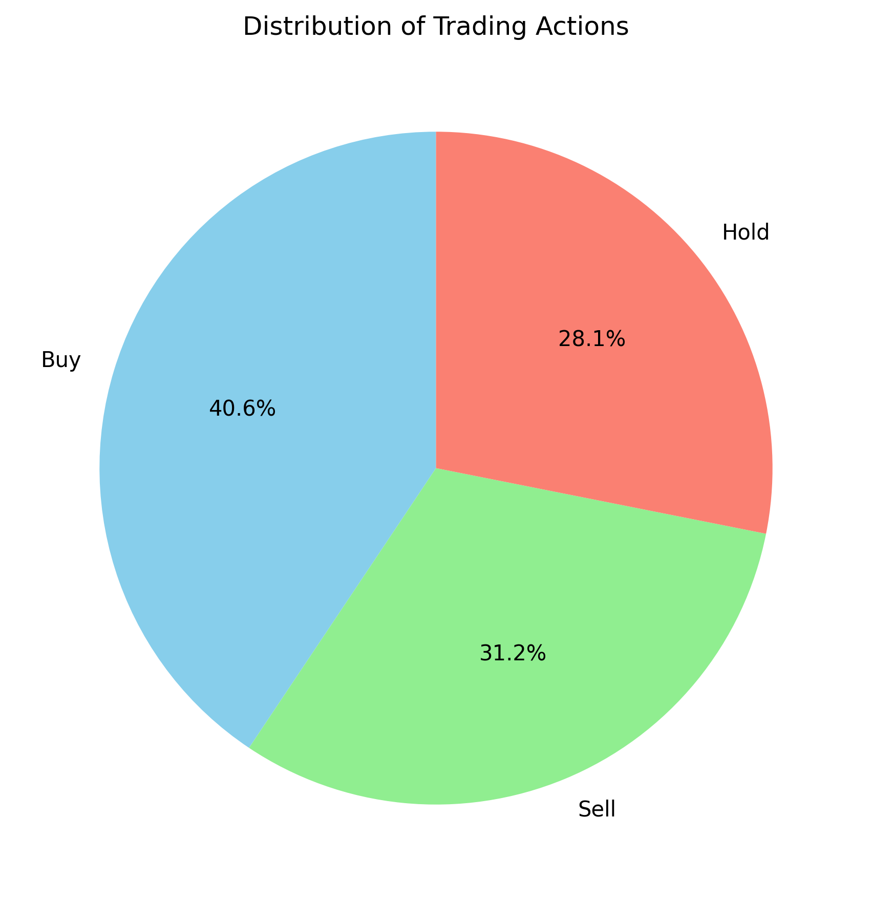
Figure A: SOFI

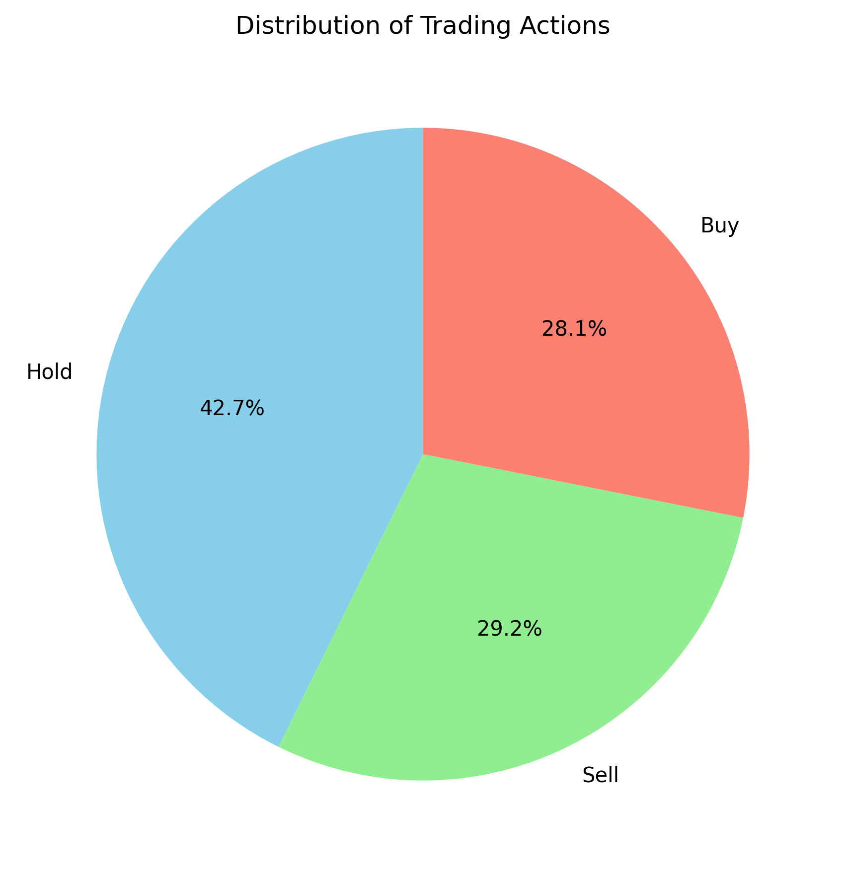
Figure B: NVDA

In this A3C model, I trained with only 100 episodes, yet it is still worth comparing the results to those from VAC. SOFI appears to behave similarly to VAC, whereas NVDA seems to make better decisions early on, as its asset value never drops below the initial amount of $10,000. However, what caught my attention is that the action distribution graphs are significantly different for the two stocks. This could be a promising direction for further investigation.