Bilateral and Guided Filters

In previous posts, we discussed basic image filters. Today, let’s move on to more advanced filters that are designed to address specific problems and purposes—namely, the Bilateral Filter and the Guided Filter. Both are examples of non-uniform smoothing filters. Let’s start with the Bilateral Filter.

Non-Uniform Smoothing: apply different smoothing degrees over areas.

Bilateral Filter

As one of the most widely used non-uniform filters, it takes into account not only spatial proximity but also differences in pixel intensity when performing averaging.

For convenience, I will compare it with the simple Gaussian Filter, which is written as follows:

$$w(i,j) \sim \exp{(-\dfrac{i^2 + j^2}{2 \cdot σ_s ^ 2})}, \space \space \space \sum_{i,j}w(i,j)=1$$

For Bilateral Filter written as:

$$w(i,j;x,y) \sim \exp{(-\dfrac{i^2 + j^2}{2 \cdot σ_s ^ 2})} \exp{(-\dfrac{|f(x+i, y+j) - f(x,y)|^2}{2 \cdot σ_r ^ 2})}, \space \space \space \sum_{i,j}w(i,j;x,y)=1$$

You can easily observe from the two formulas that the key difference lies in how the weights are assigned. The Bilateral Filter gives higher weights to pixels with more similar intensities, meaning the kernel varies from pixel to pixel. Unlike the Gaussian Filter, which only considers spatial distance, the Bilateral Filter also accounts for intensity similarity. The code is provided below:

Codebase

void gaussian_filter(Image *in, Image *out, float sigma_s, float sigma_r) {
  int W = in->getWidth();
  int H = in->getHeight();

  for (int y = 0; y < H; ++y) {
    for (int x = 0; x < W; ++x) {
      double sum = 0.0;
      double w_sum = 0.0;
      double center_value = in->get(x, y);

      for (int j = -WINSIZE; j <= WINSIZE; ++j) {
        for (int i = -WINSIZE; i <= WINSIZE; ++i) {
          int xp = x + i;
          int yp = y + j;

          if (xp < 0)
            xp = 0;
          if (xp >= W)
            xp = W - 1;
          if (yp < 0)
            yp = 0;
          if (yp >= H)
            yp = H - 1;

          double nb_val = in->get(xp, yp);
          double dist = sqrt(i * i + j * j);
          double w = exp(-(dist * dist) / (2.0 * sigma_s * sigma_s));

          w_sum += w;
          sum += w * nb_val;
        }
      }
      double val = sum / w_sum;
      out->set(x, y, val);
    }
  }
}

void bilateral_filter(Image *in, Image *out, float sigma_s, float sigma_r) {
  int W = in->getWidth();
  int H = in->getHeight();

  for (int y = 0; y < H; ++y) {
    for (int x = 0; x < W; ++x) {
      double sum = 0.0;
      double w_sum = 0.0;
      double center_value = in->get(x, y);

      for (int j = -WINSIZE; j <= WINSIZE; ++j) {
        for (int i = -WINSIZE; i <= WINSIZE; ++i) {
          int xp = x + i;
          int yp = y + j;

          if (xp < 0)
            xp = 0;
          if (xp >= W)
            xp = W - 1;
          if (yp < 0)
            yp = 0;
          if (yp >= H)
            yp = H - 1;

          double nb_val = in->get(xp, yp);

          double dist = sqrt(i * i + j * j);
          double s_w = exp(-(dist * dist) / (2.0 * sigma_s * sigma_s));

          double inten_diff = fabs(center_value - nb_val);
          double r_w =
              exp(-(inten_diff * inten_diff) / (2.0 * sigma_r * sigma_r));

          double w = s_w * r_w;

          sum += w * nb_val;
          w_sum += w;
        }
      }

      double val = sum / w_sum;
      out->set(x, y, val);
    }
  }
}

You can see how easily the code is implemented by simply adding one more term. The Bilateral Filter can be thought of as an enhanced version of the Gaussian Filter. Try setting both hyperparameters to 10 to observe the results.

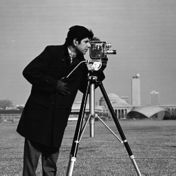
Figure 1-1: Original

Figure 1-2: Gaussian

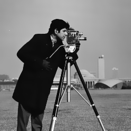
Figure 1-3: Bilateral

Clearly, the Bilateral Filter produces much better results than the other two. What intrigues me is that applying the Gaussian Filter first, followed by the Bilateral Filter, makes the entire image appear higher resolution from a purely visual perspective. This is fascinating because it suggests that sometimes introducing a bit of “messiness” can lead to a better, more refined outcome. Now, let’s dive into the Guided Filter.

Guided Filter

Compared to the Bilateral Filter, the Guided Filter has a similar goal but emphasizes faster, linear processing. Let’s look at its mathematical definition.

We want $q_i = a_kG_i + b_k$ to be as close as possible to $I_i$ (original input).

$q_i = a_kG_i + b_k$ seems weird at first, but it is based on the assumption: In a small window of an image, the ouput pixel values $q_i$ should be linearly related to the guidance image values $G_i$.

Here, $G$ means Guidance Image that could be same image, color image or any specific purpose image. Saying, G is grayscale or RGB.

1. G is grayscale: single intensity value
2. G is RGB: apply filter to each channel or use a vector formulation

In brief, you can guide the filter with any image - and that's how we give it intelligence about what features to preserve.

From the above, the objective function is to mininize:

$$E(a_{k,l},b_{k,l}) = \sum_{(x, y) \in w_{k, l}}((a_{k,l}G_{k,l} + b_{k, l} - G_{k,l})^2 + \epsilon a_{k, l}^2)$$

Tile and Intercept of objective function:

$$a_{k,l} = \dfrac{\sigma_{k,l} ^ 2}{\sigma_{k,l}^2 + \epsilon}, \space b_{k,l} = \dfrac{\epsilon}{\sigma_{k,l} ^ 2 + \epsilon}\mu_{k,l}$$

where:

• $\mu_{k,l} = \dfrac{1}{|W|}\sum_{(x,y) \in W_{k,l}}G(x,y)$
• $\sigma_{k,l}^2 = \dfrac{1}{|W|}\sum_{(x,y) \in W_{k,l}} |G(x,y) - \mu_{k,l}|^2$

Carefully derived above, the simpler form is obtained and written as:

$$O(x,y) = \dfrac{1}{|W|} \sum_{(x,y) \in W_{k,l}} a_{k,l}G(x,y) + b_{k,l} \\ = \bar{a} (x,y)G(x,y) + \bar{b} (x,y)$$

We will implement it approximately as

$$a_{k,l}I(x,y) + b_{k,l} \approx I(x,y) or \approx \mu_{k,l}$$

based on the size of $a_{k,l}^2$ is large or small.

Code is given as follows:

void guided_filter(Image *in, Image *out, float eps, float r) {
  int W = in->getWidth();
  int H = in->getHeight();
  int C = in->getCH();

  for (int y = 0; y < H; ++y) {
    for (int x = 0; x < W; ++x) {
      int window_count = 0;
      double window_sum = 0.0;
      double window_sum_sq = 0.0;

      for (int j = -WINSIZE / 2; j <= WINSIZE / 2; ++j) {
        for (int i = -WINSIZE / 2; i <= WINSIZE / 2; ++i) {
          int xp = x + i;
          int yp = y + j;

          if (xp < 0)
            xp = 0;
          if (xp >= W)
            xp = W - 1;
          if (yp < 0)
            yp = 0;
          if (yp >= H)
            yp = H - 1;

          double nb_val = in->get(xp, yp);
          window_sum += nb_val;
          window_sum_sq += nb_val * nb_val;
          window_count++;
        }
      }

      double window_avg = window_sum / window_count;
      double window_var =
          (window_sum_sq / window_count) - (window_avg * window_avg);

      double tilt = window_var / (window_var + eps);
      double intercept = window_avg - tilt * window_avg;

      double center_value = in->get(x, y);
      double filtered_value = tilt * center_value + intercept;

      filtered_value = std::max(0.0, std::min(255.0, filtered_value));
      out->set(x, y, filtered_value);
    }
  }
}

Let's view the results.

Figure 2-1: Original

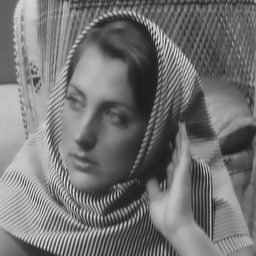
Figure 2-2: Guided

The Guided Filter seems to be working as expected. Just make sure to clamp the pixel values in the code to stay within the valid range, in case they fall below 0 or exceed 255.

Conclusion

We’ve learned two more filters in image processing. These are significantly more complex than the filters we discussed previously, as they rely on the statistical properties of image pixels. They fundamentally change the way we think about images and visual data. I believe there is still much to discover in this area of research. Interestingly, it connects with my recent work in reinforcement learning (RL) and evolutionary strategies (ES), providing new perspectives and possible directions for exploration.