Binarization and Error Diffusion

In the previous post, we discussed Image Filter and Edge Detection.

Today, let’s explore another fundamental and essential topic in image processing: binarization. This concept plays a critical role in many advanced image processing techniques and lays the groundwork for tasks such as object recognition, text extraction, and pattern analysis.

Binarization Introduction

As you might know, "binary" refers to two values — typically 0 and 1.

In the context of image processing, binarization follows the same principle: converting an image into a binary format where each pixel is represented by only two possible values, usually 0 (black) and 255 (white). This simplification is especially useful for tasks like text recognition, shape analysis, and image segmentation.

• 0: black
• 1: white

At first glance, converting all pixels in an image to just 0 or 1 might seem meaningless — after all, wouldn’t that just result in a completely black or white image? You're actually close to the core idea of binarization, but there's one critical element to consider: the threshold.

By applying a threshold, we determine which pixels should become white (1 or 255) and which should become black (0). This concept is similar to the step function used in neural networks or on-off control in control engineering. Even in simple Laplace transformations, the idea of binary decision-making plays a foundational role. In all these cases, we’re classifying values based on whether they are above or below a certain threshold.

The binarization process can be defined as follows:

$$I_{binary}(x, y) = \begin{cases} 0, \space \text{If} (x, y) < T \\ 255, \text{otherwise} \end{cases}$$

But why do we need to binarize an image in the first place? Here are a few key reasons:

1. Simplification: reduces image complexity helps to perform other tasks like shape recognition or contour finding.
2. Feature Extraction: binarized text is easier to separate from background noice such as OCR (Optical Character Recognition).
3. Noise Reduction: acts as a preliminary step for morphological operations.

There are several types of binarization methods that use different ways to determine the threshold. Here are some common approaches:

1. Fixed Thresholding (T = 127): simple but sensitive to lighting variation.
2. Adaptive Thresholding: threshold is computed based on each small region.
3. Otsu's Thresholding: automatically choose the threshold to minimize intra-class variance.

For this post, we’ll focus on fixed thresholding and see how it works in practice. Below is a simple example code demonstrating this method:

Binarization Implementation

void binarization_fixed_threshold(
  Image *in, Image *out, double threshold) {
  int W = in->getWidth();
  int H = in->getHeight();
  int C = in->getCH();

  for (int y = 0; y < H; ++y) {
    for (int x = 0; x < W; ++x) {
      if (C == 1) {
        double val_in = in->get(x, y);
        double val_out = 0.0;

        if (val_in > threshold)
          val_out = 255.0;

        out->set(x, y, val_out);
      } else {
        double r_value = in->get(x, y, 0);
        double g_value = in->get(x, y, 1);
        double b_value = in->get(x, y, 2);

        if (r_value > threshold)
          r_value = 255.0;
        else
          r_value = 0.0;

        if (g_value > threshold)
          g_value = 255.0;
        else
          g_value = 0.0;

        if (b_value > threshold)
          b_value = 255.0;
        else
          b_value = 0.0;

        out->set(x, y, 0, r_value);
        out->set(x, y, 1, g_value);
        out->set(x, y, 2, b_value);
      }
    }
  }
}

In this example, I also consider the color channels individually. For grayscale images, since there is only one channel, the thresholding is applied directly to that channel.

The process is simple: for each pixel, check if its value is greater than the threshold. If it is, set the pixel to 255 (white); otherwise, set it to 0 (black).

Below are the results of applying different fixed threshold values — 32, 64, and 127 — to both grayscale and RGB images for comparison.

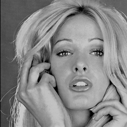
Figure 1-1: Original

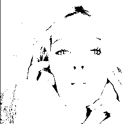
Figure 1-2: T = 64

Figure 1-3: T = 127

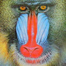
Figure 2-1: Original

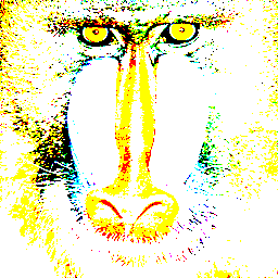
Figure 2-2: T = 64

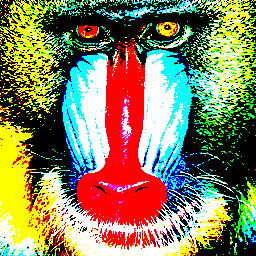
Figure 2-3: T = 127

Now that we understand fixed threshold binarization, it’s important to note its limitation: using a single threshold often causes significant information loss, as many subtle details are discarded. To address this issue, there are alternative techniques designed to preserve more information. One such approach is Error Diffusion, which helps maintain image detail even after binarization.

Error Diffusion Introduction

Error Diffusion is a technique commonly used in halftoning and binary image conversion that aims to preserve as much visual detail as possible. In short, this method propagates the quantization error of a pixel to its neighboring pixels within a defined area. By distributing the error, it reduces the harsh effects of simple thresholding and produces a more visually pleasing binary image.

1. Rounding each pixel to either 0 or 255.
2. Calculating the error between the original image and the binary value.
3. Distributing (diffusing) this error to neighboring pixels.

The core of error diffusion lies in the third step, where the quantization error of the current pixel is distributed to its neighboring pixels. This process adjusts the brightness of surrounding pixels, helping to preserve the overall brightness and visual texture of the image.

$$ε = I(x,y) - B(x,y)$$

• $I(x,y)$: pixel value
• $B(x,y)$: binary output of a pixel value

Diffusion Kernel (aka. Floyd-Steinberg)

$$\begin{bmatrix} * & * & \text{pixel} & \dfrac{7}{16} \\ * & \dfrac{3}{16} & \dfrac{5}{16} & \dfrac{1}{16} \end{bmatrix}$$

This kernel distributes the quantization error to neighboring pixels, effectively acting as an error smoothing technique that helps preserve image details and reduces harsh binarization artifacts.

const int ERROR_DIFFUTION_DIRS[4][2] = {
  {1, 0}, {0, 1}, {-1, 1}, {1, 1}};
const int ERROR_DIFFUTION_WEIGHTS[4] = {7, 5, 3, 1};
const float ERROR_DIFFUTION_SUM = 16.0;

void binarization_error_diffusion(
  Image *in, Image *out, double threshold) {
  int W = in->getWidth();
  int H = in->getHeight();
  int C = in->getCH();

  for (int y = 0; y < H; ++y) {
    for (int x = 0; x < W; ++x) {
      if (C == 1) {
        double val_in = in->get(x, y);
        double val_out = val_in > threshold ? 255.0 : 0.0;
        double error = val_in - val_out;
        out->set(x, y, val_out);
        for (int p = 0; p < 4; ++p) {
          int dx = ERROR_DIFFUTION_DIRS[p][0];
          int dy = ERROR_DIFFUTION_DIRS[p][1];
          int xp = x + dx;
          int yp = y + dy;

          if (xp < 0 || xp >= W || yp < 0 || yp >= H)
            continue;

          double neighbor_in_value = in->get(xp, yp);
          neighbor_in_value +=
              error * ERROR_DIFFUTION_WEIGHTS[p] / ERROR_DIFFUTION_SUM;
          in->set(xp, yp, neighbor_in_value);
        }
      } else {
        double val_r_in = in->get(x, y, 0);
        double val_g_in = in->get(x, y, 1);
        double val_b_in = in->get(x, y, 2);

        double val_r_out = val_r_in > threshold ? 255.0 : 0.0;
        double val_g_out = val_g_in > threshold ? 255.0 : 0.0;
        double val_b_out = val_b_in > threshold ? 255.0 : 0.0;

        out->set(x, y, 0, val_r_out); // Set binarized R
        out->set(x, y, 1, val_g_out); // Set binarized G
        out->set(x, y, 2, val_b_out); // Set binarized B

        double error_r = val_r_in - val_r_out;
        double error_g = val_g_in - val_g_out;
        double error_b = val_b_in - val_b_out;

        for (int p = 0; p < 4; ++p) {
          int dx = ERROR_DIFFUTION_DIRS[p][0];
          int dy = ERROR_DIFFUTION_DIRS[p][1];
          int xp = x + dx;
          int yp = y + dy;

          if (xp < 0 || xp >= W || yp < 0 || yp >= H)
            continue;

          double val_r_in = in->get(xp, yp, 0);
          double val_g_in = in->get(xp, yp, 1);
          double val_b_in = in->get(xp, yp, 2);
          val_r_in +=
              error_r * ERROR_DIFFUTION_WEIGHTS[p] / ERROR_DIFFUTION_SUM;
          val_g_in +=
              error_g * ERROR_DIFFUTION_WEIGHTS[p] / ERROR_DIFFUTION_SUM;
          val_b_in +=
              error_b * ERROR_DIFFUTION_WEIGHTS[p] / ERROR_DIFFUTION_SUM;

          in->set(xp, yp, 0, val_r_in);
          in->set(xp, yp, 1, val_g_in);
          in->set(xp, yp, 2, val_b_in);
        }
      }
    }
  }
}

Figure 3-1: Original

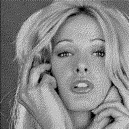
Figure 3-2: T = 127

Figure 3-3: T = 255

Figure 4-1: Original

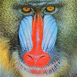
Figure 4-2: T = 127

Figure 4-3: T = 255

From these images, you can observe that error diffusion is much less sensitive to the choice of threshold value. In simple terms, the threshold doesn’t significantly affect the final output because the error diffusion process continuously self-corrects, balancing the tonal information throughout the image. You can find the codebase here.

Conclusion

So far, we’ve explored two image processing techniques and observed their visual differences. What intrigues me is how these methods share common principles with approaches I’ve encountered in machine learning.

This insight sparks exciting possibilities — for example, could similar techniques be applied in reinforcement learning? Could we propagate rewards or states in a way that smooths out policy errors, much like error diffusion smooths image details?

These ideas are definitely worth exploring. It’s both exciting and thrilling to see connections like these across different fields!