Deconvolution

Over the past few days, we have covered many topics related to image processing. In particular, the first few posts focused on applying various image filters using kernel convolution. Today, it’s time to explore how to apply deconvolution to these filtered images. So, what exactly is deconvolution? Here is a brief overview:
- Invert Kernel Convolution
- Applications:
- Blur Removal: camera shake, optical blur, motion blur and etc.
- Super-resolution: integrate several low-resolution images.
- Non-blind/blind Deconvolution
- Kernel is known (non-blind) or not (blind)
For 1-D signal, the process looks like this:
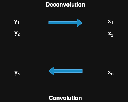
This process, defined as a linear transformation, can be easily formulated as follows:
$$\begin{pmatrix} y_1 \\ y_2 \\ \vdots \\ y_n \end{pmatrix} = \dfrac{1}{3} \begin{pmatrix} 1 & 1 & 0 & \cdots & 0 & 1 \\ 1 & 1 & 1 & \ddots & 0 & 0 \\ 0 & \ddots & \ddots & \ddots & \ddots & \vdots \\ \vdots & \ddots & \ddots & \ddots & \ddots & 0 \\ 0 & \ddots & \ddots & 1 & 1 & 1 \\ 1 & 0 & \cdots & 0 & 1 & 1 \end{pmatrix} \begin{pmatrix} x_1 \\ x_2 \\ \vdots \\ x_n \end{pmatrix}$$
However, the inverse of the convolution matrix generally does not exist, and even when it does, computing the inverse is often computationally expensive. As a result, we typically use the Least Squares Method (LSM) to approximate the solution. The deconvolution problem can be formulated as follows:
Least Sequare Method
$$\argmin_{x} |y - Ax|^2$$
Gradient Decent
- Objective Function: $E(x) = \dfrac{1}{2} |y - Ax|^2$
- Gradient: $\nabla E(x) = -A^T(y - Ax)$
- Update Rule: $x^{t+1} = x^t - \alpha^t \nabla E(x^t), \quad \alpha^t = \dfrac{|\nabla E(x^t)| ^ 2}{A|\nabla E(x^t)| ^ 2}$
In this post, we will use kernels from Image Filter and Edge Detection —such as the Gaussian filter, horizontal edge filter, and Laplacian filter—and apply deconvolution to the corresponding filtered images. Below is the pseudocode for this operation.
$$\begin{align} & \textbf{Input: } Y \text{ (blurry image)} \\ &X \leftarrow Y \\ &\textbf{repeat} \\ & \quad G \leftarrow -b(Y - b(X)) \\ & \quad \alpha \leftarrow \dfrac{||G||^2}{||b \cdot G||^2} \\ & \quad X \leftarrow X - \alpha G \\ & \textbf{until convergence} \\ & \textbf{Output: } X\end{align}$$
In this post, we focus exclusively on non-blind deconvolution, where the kernel is known in advance.
double GAUSSIAN_K[3][3] = {{1.0 / 16.0, 2.0 / 16.0, 1.0 / 16.0},
                           {2.0 / 16.0, 4.0 / 16.0, 2.0 / 16.0},
                           {1.0 / 16.0, 2.0 / 16.0, 1.0 / 16.0}};
const int SOBEL_HRZ_K[3][3] = {{-1, 0, 1}, {-2, 0, 2}, {-1, 0, 1}};
const int LAPLACIAN_K_DIAG[3][3] = {{1, 1, 1}, {1, -8, 1}, {1, 1, 1}};

void deconvolution_gaussian(Image *in, Image *out) {
  int W = in->getWidth();
  int H = in->getHeight();
  int C = in->getCH();

  printf("Starting Gaussian/Mean Filter Deconvolution...\n");

  for (int y = 0; y < H; ++y) {
    for (int x = 0; x < W; ++x) {
      out->set(x, y, in->get(x, y));
    }
  }

  int max_iterations = 1000;
  double tolerance = 1e-4;
  double prev_objective = 1e10;
  double lambda = 0.001;

  Image *Ax = new Image();
  Image *A_grad = new Image();
  Image *residual = new Image();
  Image *gradient = new Image();

  Ax->init(W, H, 1);
  A_grad->init(W, H, 1);
  residual->init(W, H, 1);
  gradient->init(W, H, 1);

  int iter = 0;
  while (iter < max_iterations) {
    double mse = 0.0;
    double reg_term = 0.0;

    // Compute A*x using Gaussian kernel
    for (int y = 0; y < H; ++y) {
      for (int x = 0; x < W; ++x) {
        double sum = 0.0;

        for (int ky = -1; ky <= 1; ++ky) {
          for (int kx = -1; kx <= 1; ++kx) {
            int px = x + kx;
            int py = y + ky;

            if (px < 0)
              px += W;
            if (px >= W)
              px -= W;
            if (py < 0)
              py += H;
            if (py >= H)
              py -= H;

            sum += GAUSSIAN_K[ky + 1][kx + 1] * out->get(px, py);
          }
        }

        Ax->set(x, y, sum);
      }
    }

    for (int y = 0; y < H; ++y) {
      for (int x = 0; x < W; ++x) {
        residual->set(x, y, in->get(x, y) - Ax->get(x, y));
        mse += residual->get(x, y) * residual->get(x, y);

        double x_val = out->get(x, y);
        reg_term += lambda * x_val * x_val;
      }
    }

    double current_objective = mse / 2.0 + reg_term / 2.0;

    for (int y = 0; y < H; ++y) {
      for (int x = 0; x < W; ++x) {
        double sum = 0.0;

        for (int ky = -1; ky <= 1; ++ky) {
          for (int kx = -1; kx <= 1; ++kx) {
            int px = x - kx;
            int py = y - ky;

            if (px < 0)
              px += W;
            if (px >= W)
              px -= W;
            if (py < 0)
              py += H;
            if (py >= H)
              py -= H;

            sum += GAUSSIAN_K[(-ky) + 1][(-kx) + 1] \
              * residual->get(px, py);
          }
        }

        gradient->set(x, y, -sum + lambda * out->get(x, y));
      }
    }

    double grad_norm_sq = 0.0;
    for (int y = 0; y < H; ++y) {
      for (int x = 0; x < W; ++x) {
        double g = gradient->get(x, y);
        grad_norm_sq += g * g;
      }
    }

    if (sqrt(grad_norm_sq) < tolerance) {
      printf("Converged after %d iterations (gradient norm: %e)\n", iter,
             sqrt(grad_norm_sq));
      break;
    }

    if (iter > 0 &&
        (prev_objective - current_objective) / prev_objective < 1e-6) {
      printf("Converged after %d iterations (minimal improvement)\n",
        iter);
      break;
    }

    prev_objective = current_objective;

    // Compute optimal step size
    for (int y = 0; y < H; ++y) {
      for (int x = 0; x < W; ++x) {
        double sum = 0.0;

        for (int ky = -1; ky <= 1; ++ky) {
          for (int kx = -1; kx <= 1; ++kx) {
            int px = x + kx;
            int py = y + ky;

            if (px < 0)
              px += W;
            if (px >= W)
              px -= W;
            if (py < 0)
              py += H;
            if (py >= H)
              py -= H;

            sum += GAUSSIAN_K[ky + 1][kx + 1] * gradient->get(px, py);
          }
        }

        A_grad->set(x, y, sum);
      }
    }

    double A_grad_norm_sq = 0.0;
    for (int y = 0; y < H; ++y) {
      for (int x = 0; x < W; ++x) {
        double ag = A_grad->get(x, y);
        A_grad_norm_sq += ag * ag;
      }
    }

    double denominator = A_grad_norm_sq + lambda * grad_norm_sq;
    if (denominator > 1e-12) {
      alpha = grad_norm_sq / denominator;
    } else {
      alpha = 0.001;
    }

    if (alpha > 0.1)
      alpha = 0.1;
    if (alpha < 1e-6)
      alpha = 1e-6;

    for (int y = 0; y < H; ++y) {
      for (int x = 0; x < W; ++x) {
        double new_val = out->get(x, y) - alpha * gradient->get(x, y);
        if (new_val > 255.0)
          new_val = 255.0;
        if (new_val < 0.0)
          new_val = 0.0;
        out->set(x, y, new_val);
      }
    }

    if (iter % 10 == 0) {
      printf("--------------------------------\n");
      printf("Iteration: %d\n", iter);
      printf("Objective Function: %f (Data: %f, Reg: %f)\n",
        current_objective,
        mse / 2.0, reg_term / 2.0);
      printf("Gradient Norm: %e\n", sqrt(grad_norm_sq));
      printf("Alpha: %f\n", alpha);
      printf("--------------------------------\n");
    }

    iter++;
  }

  if (iter >= max_iterations) {
    printf("Reached maximum iterations (%d) without full convergence\n",
           max_iterations);
  }

  delete Ax;
  delete residual;
  delete gradient;
  delete A_grad;
}
Gaussian Filter Deconvolution - CSY
From the code, we can compare how deconvolution behaves when applied to an image filtered with a mean filter.

Figure 1-1: Original

Figure 1-2: Gaussian

Figure 1-3: Deconvolution
We can observe that deconvolution is effective in this case, as applying it to the filtered image successfully restores the original image, albeit with some noise. However, when the same process is applied to images filtered with mean, Sobel, or Laplacian kernels, it fails to restore the original. This is because these filters cause irreversible data loss, making perfect reconstruction impossible.
Figure 1-1: Original

Figure 1-2: Mean Filtered
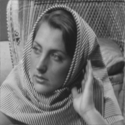
Figure 1-3: Deconvolution
Figure 2-1: Original
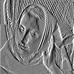
Figure 2-2: Sobel
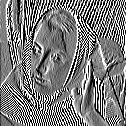
Figure 2-3: Deconvolution
Figure 3-1: Original
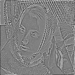
Figure 3-2: Laplacian
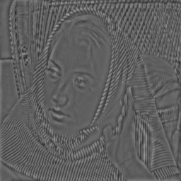
Figure 3-3: Deconvolution
Conclusion
Based on the implementation and generated images above, we can conclude that only transformations that retain essential information—i.e., those that are invertible or nearly invertible—can be effectively reversed through deconvolution.
Gaussian blur, for example, is recoverable because it merely disperses pixel intensities without discarding information. From a linear algebra perspective, such transformations are considered full-rank.
In short, deconvolution can recover what has been blurred, but not what has been lost.


