Frequency Analysis

One of the most important topics in image processing is frequency analysis, which offers a completely new perspective for understanding images. Unlike the spatial domain, frequency analysis examines images in the frequency domain, allowing us to uncover underlying patterns that are especially useful for tasks such as filtering, compression, and enhancement.
In general, an image can be analyzed in two main domains:
- Spatial Domain: where images are represented by pixel intensity values.
- Frequency Domain: where we analyze how pixel intensity values change over space.
To shift from the spatial to the frequency domain, we use the Fourier Transform (FT) — more specifically, the Discrete Fourier Transform (DFT) for digital images. This mathematical transformation converts an image’s spatial information into its frequency components.
The 2D DFT for an image is defined as follows:
$$F(u,v) = \sum_{x=0}^{M-1} \sum_{y=0}^{N-1} f(x,y) e^{-j2π(\dfrac{ux}{M} + \dfrac{vu}{N})}$$
- $f(x,y)$: pixel intensity
- $F(u,v)$: frequency representation of image
- $u,v$: frequency coordinates
In the frequency domain, different frequency components carry distinct meanings:
- Low Frequencies: correspond to smooth areas in the image, where intensity values change gradually.
- High Frequencies: represent sharp transitions, such as edges, noise, or fine textures.
To perform frequency analysis on images, we apply the Fourier Transform. Since images are two-dimensional, we use a 1D Fast Fourier Transform (FFT) sequentially along two axes — first across rows (horizontal), and then down columns (vertical). This approach efficiently computes the 2D FFT by leveraging the separability of the transform.
Among various FFT algorithms, the most widely used is the Cooley-Tukey FFT algorithm.
Cooley-Turkey FFT
A divide-and-conquer algorithm that reduce time complexity from $O(N^2)$ to $O(N \log N)$.
If N is even, split the input singal into even and odd-indexed elements.
$$X[k] = \sum_{n=0}^{N/2 - 1} x[2n]e^{-j\dfrac{2πkn}{N/2}} + e^{-j\dfrac{2πk}{N}} \cdot \sum_{n=0}^{N/2-1} x[2n+1]e^{-j\dfrac{2πkn}{N/2}}$$
- $E[k]$: FFT of even-indexed elements
- $O[k]$: FFT of odd-indexed elements
- $W_N^k = e^{-j\dfrac{2πk}{N}}$: Twiddle factor
The code is provided as follows:
void cooley_tukey_fourier(
    double data[], unsigned long nn, int isign) {

  // data[]: Input/Output array of size 2 * nn
  //   data[2i]: real part
  //   data[2i+1]: imaginary part
  // nn: Number of complex points
  // isign: Direction of transform (1: forward FFT, -1: inverse FFT)

  unsigned long n, mmax, m, j, istep, i;

  double wtemp, wr, wpr, wpi, wi, theta;
  double tempr, tempi;

  n = nn << 1;
  j = 1;

  // Bit-Reversal Permutation
  for (i = 1; i < n; i += 2) {
    if (j > i) {
      SWAP(data[j], data[i]);
      SWAP(data[j + 1], data[i + 1]);
    }

    m = n >> 1;
    while (m >= 2 && j > m) {
      j -= m;
      m >>= 1;
    }
    j += m;
  }

  // FFT Main Loop
  mmax = 2; # Size of the current sub-DFT being merged
  while (n > mmax) {
    istep = mmax << 1;
    theta = isign * (M_PI * 2 / mmax); # Rotation angle
    wtemp = sin(0.5 * theta);
    wpr = -2.0 * wtemp * wtemp;
    wpi = sin(theta);
    wr = 1.0;
    wi = 0.0;
    for (m = 1; m < mmax; m += 2) {
      for (i = m; i <= n; i += istep) {
        j = i + mmax;
        tempr = wr * data[j] - wi * data[j + 1];
        tempi = wr * data[j + 1] + wi * data[j];
        data[j] = data[i] - tempr;
        data[j + 1] = data[i + 1] - tempi;
        data[i] += tempr;
        data[i + 1] += tempi;
      }
      wr = (wtemp = wr) * wpr - wi * wpi + wr;
      wi = wi * wpr + wtemp * wpi + wi;
    }
    mmax = istep;
  }

  if (isign == -1) {
    for (i = 1; i <= n; ++i) {
      data[i] /= nn;
    }
  }
}
Cooley-Turkey FFT - CSY
Fourier Transform
Once the 1D FFT has been applied across both the horizontal and vertical directions, we obtain the image representation in the frequency domain. From this complex-valued result, we can extract two key components:
- Amplitude (or Magnitude) Spectrum: Represents the strength of different frequency components. It highlights where the dominant structures or patterns in the image exist.
$$\text{Amplitude}(u,v) = \sqrt{Re(F(u,v))^2 + Im(F(u,v))^2}$$
- Phase Spectrum: Encodes the positional information of structures in the image. Even though it may look abstract, it is crucial for accurately reconstructing the original image.
$$\text{Phase}(u,v) = \tan^{-1}{\dfrac{Im(F(u,v))}{Re(F(u,v))}}$$
#define MAXSIZE 1024

void fourier_transform_amplitude(Image *in, Image *out) {

  int W = in->getWidth();
  int H = in->getHeight();

  Image *re_img = new Image(); // real part
  Image *im_img = new Image(); // imaginary part
  re_img->init(W, H, 1);
  im_img->init(W, H, 1);

  int x, y;

  // ----- 2D Fourier Transform
  double data[MAXSIZE + 1];

  // Horizontal direction
  for (y = 0; y < H; ++y) {
    int m;
    for (x = 0; x < W; ++x) {
      m = x * 2 + 1;
      data[m] = in->get(x, y); // real part = pixel value
      data[m + 1] = 0;         // imaginary part = 0
    }
    cooley_tukey_fourier(data, W, 1);
    for (x = 0; x < W; ++x) {
      m = x * 2 + 1;
      re_img->set(x, y, data[m]);
      im_img->set(x, y, data[m + 1]);
    }
  }

  // Vertical direction
  for (x = 0; x < W; ++x) {
    int m;
    for (y = 0; y < H; ++y) {
      m = y * 2 + 1;
      data[m] = re_img->get(x, y);
      data[m + 1] = im_img->get(x, y);
    }
    cooley_tukey_fourier(data, H, 1);
    for (y = 0; y < H; ++y) {
      m = y * 2 + 1;
      re_img->set(x, y, data[m]);
      im_img->set(x, y, data[m + 1]);
    }
  }

  Image *amp = new Image();
  amp->init(W, H, 1);

  for (x = 0; x < W; ++x) {
    for (y = 0; y < H; ++y) {
      double re, im;
      re = re_img->get(x, y);
      im = im_img->get(x, y);

      double amplitude;
      amplitude = sqrt(re * re + im * im);
      amp->set(x, y, amplitude);
    }
  }

  Image *amp_c = new Image();
  amp_c->init(W, H, 1);
  for (x = 0; x < W; x++) {
    for (y = 0; y < H; y++) {
      double amp_value;
      int m, n;
      amp_value = amp->get(x, y);
      m = (W / 2 + x) % W;
      n = (H / 2 + y) % H;
      amp_c->set(m, n, amp_value);
    }
  }

  // Find maximum value
  double max_amp = 0.0;
  for (x = 0; x < W; ++x) {
    for (y = 0; y < H; ++y) {
      double tmp = amp_c->get(x, y);
      if ((tmp > max_amp)) {
        max_amp = tmp;
      }
    }
  }

  for (x = 0; x < W; ++x) {
    for (y = 0; y < H; ++y) {
      double tmp = amp_c->get(x, y);
      int value = int(log(tmp) / log(max_amp) * 255.0);
      out->set(x, y, value);
    }
  }
}
FFT Amplitude - CSY
For the phase image, the procedure remains the same as for the amplitude image — the only difference lies in how the phase is computed from the FFT result.
void fourier_transform_phase(Image *in, Image *out) {
  int W = in->getWidth();
  int H = in->getHeight();

  Image *re_img = new Image(); // real part
  Image *im_img = new Image(); // imaginary part
  re_img->init(W, H, 1);
  im_img->init(W, H, 1);

  int x, y;

  // ----- 2D Fourier Transform
  double data[MAXSIZE + 1];

  // Horizontal direction
  for (y = 0; y < H; ++y) {
    int m;
    for (x = 0; x < W; ++x) {
      m = x * 2 + 1;
      data[m] = in->get(x, y); // real part = pixel value
      data[m + 1] = 0;         // imaginary part = 0
    }
    cooley_tukey_fourier(data, W, 1);
    for (x = 0; x < W; ++x) {
      m = x * 2 + 1;
      re_img->set(x, y, data[m]);
      im_img->set(x, y, data[m + 1]);
    }
  }

  // Vertical direction
  for (x = 0; x < W; ++x) {
    int m;
    for (y = 0; y < H; ++y) {
      m = y * 2 + 1;
      data[m] = re_img->get(x, y);
      data[m + 1] = im_img->get(x, y);
    }
    cooley_tukey_fourier(data, H, 1);
    for (y = 0; y < H; ++y) {
      m = y * 2 + 1;
      re_img->set(x, y, data[m]);
      im_img->set(x, y, data[m + 1]);
    }
  }

  Image *phase = new Image();
  phase->init(W, H, 1);

  for (x = 0; x < W; ++x) {
    for (y = 0; y < H; ++y) {
      double re = re_img->get(x, y);
      double im = im_img->get(x, y);

      double phase_value = atan2(im, re) * 180.0 / M_PI;
      phase->set(x, y, phase_value);
    }
  }

  Image *phase_c = new Image();
  phase_c->init(W, H, 1);
  for (x = 0; x < W; ++x) {
    for (y = 0; y < H; ++y) {
      double phase_value = phase->get(x, y);
      int m = (W / 2 + x) % W;
      int n = (H / 2 + y) % H;
      phase_c->set(m, n, phase_value);
    }
  }

  for (x = 0; x < W; ++x) {
    for (y = 0; y < H; ++y) {
      double tmp = phase_c->get(x, y);
      int value = int((tmp + 180.0) / 360.0 * 255.0);
      out->set(x, y, value);
    }
  }
}
FFT Phase - CSY
Of course, we can perform this entire procedure — including computing both amplitude and phase — within a single function. However, the reason I separate the steps here is to clearly highlight each component of the concept. By isolating the operations, it becomes easier to understand the role of each part in the frequency domain.
Now, let’s take a look at the results below.
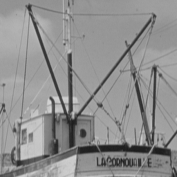
Figure 1-1: Original
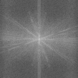
Figure 1-2: Amplitude
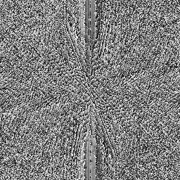
Figure 1-3: Phase
Note: Before saving the amplitude and phase images in PGM format, we need to normalize their values to the range [0,255] , as this is the standard requirement for grayscale image formats.
Inverse-FFT
This step converts the image from the frequency domain back to the spatial domain. Since we previously split the image into amplitude and phase, we now need to recombine these two components to reconstruct the original image.
$$x[n] = IFFT(X[k]) $$
- $x[n]$: original singal
- $X[k] = FFT(x[n])$: frequency domain information
$$x[n] = \dfrac{1}{N} \sum_{k=0}^{N-1} X[k] \cdot e^{+j2πkn/N}$$
void inverse_fourier_transform(
    Image *amp_in, Image *phase_in, Image *out) {

  double data[MAXSIZE + 1]; // Caution: The index starts from 1.

  int x, y;
  int W = amp_in->getWidth();
  int H = amp_in->getHeight();

  Image *amp_c = new Image();
  Image *phase_c = new Image();
  amp_c->init(W, H, 1);
  phase_c->init(W, H, 1);

  for (x = 0; x < W; x++) {
    for (y = 0; y < H; y++) {
      int amp_value = amp_in->get(x, y);
      // Inverse of amplitude value = int(log(tmp)/log(maxamp)*255.0);
      double amp_tmp = exp(amp_value / 255.0 * log(MAXAMP));
      amp_c->set(x, y, amp_tmp);

      int phase_value = phase_in->get(x, y);
      // Inverse of phase value = int((tmp + 180.0)/360.0*255.0);
      double phase_tmp = (phase_value / 255.0 * 360.0) - 180.0;
      phase_c->set(x, y, phase_tmp);
    }
  }

  // ----- Move DC from the center to the top-left. <==== Point 1 !!
  Image *amp = new Image();   // amplitude
  Image *phase = new Image(); // phase
  amp->init(W, H, 1);
  phase->init(W, H, 1);
  for (x = 0; x < W; x++) {
    for (y = 0; y < H; y++) {
      double amp_value = amp_c->get(x, y);
      double phase_value = phase_c->get(x, y);

      int m, n;
      m = (W / 2 + x) % W;
      n = (H / 2 + y) % H;
      amp->set(m, n, amp_value);
      phase->set(m, n, phase_value);
    }
  }

  // Calculate (re, im) image
  Image *re_img = new Image(); // real part
  Image *im_img = new Image(); // imaginary part
  re_img->init(W, H, 1);
  im_img->init(W, H, 1);
  for (x = 0; x < W; x++) {
    for (y = 0; y < H; y++) {
      double re, im;
      double amplitude = amp->get(x, y);
      double phase_value = phase->get(x, y) * M_PI / 180.0;

      re = amplitude * cos(phase_value);
      im = amplitude * sin(phase_value);

      re_img->set(x, y, re);
      im_img->set(x, y, im);
    }
  }

  // ----- 2D Inverse Fourier Transform
  // Horizontal direction
  for (y = 0; y < H; y++) {
    int m;
    for (x = 0; x < W; x++) {
      m = x * 2 + 1;
      data[m] = re_img->get(x, y);
      data[m + 1] = im_img->get(x, y);
    }
    cooley_tukey_fourier(data, W, -1); // Inverse!
    for (x = 0; x < W; x++) {
      m = x * 2 + 1;
      re_img->set(x, y, data[m]);
      im_img->set(x, y, data[m + 1]);
    }
  }

  // Vertical direction
  for (x = 0; x < W; x++) {
    int m;
    for (y = 0; y < H; y++) {
      m = y * 2 + 1;
      data[m] = re_img->get(x, y);
      data[m + 1] = im_img->get(x, y);
    }
    cooley_tukey_fourier(data, H, -1); // Inverse
    for (y = 0; y < H; y++) {
      m = y * 2 + 1;
      re_img->set(x, y, data[m]);
      im_img->set(x, y, data[m + 1]);
    }
  }

  for (x = 0; x < W; x++) {
    for (y = 0; y < H; y++) {
      int value = re_img->get(x, y);
      out->set(x, y, value);
    }
  }

  delete amp;
  delete phase;
  delete amp_c;
  delete phase_c;
  delete re_img;
  delete im_img;
}
Inverse FFT - CSY
If we apply the inverse FFT using the amplitude and phase from the same image, we can successfully reconstruct the original image.
However, to make things more interesting, we can try combining the amplitude from one image with the phase from another. This reveals how each component contributes to the final reconstruction — and you'll often find that the phase plays a surprisingly dominant role in preserving structural details.
Figure 2-1: Boat
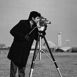
Figure 2-2: Cameraman
Figure 3-1: Boat Amplitude
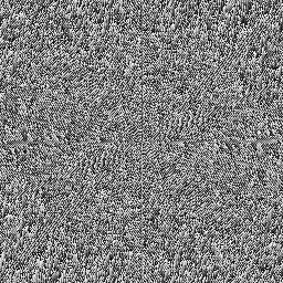
Figure 3-2: Cameraman Phase
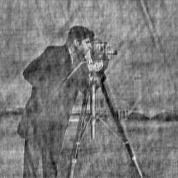
Figure 3-3: Combined
Now you can see how the Fourier Transform works and some of its intriguing properties. This is just a glimpse of its full potential. For example, since most of the energy in the amplitude spectrum is concentrated near the center, we can apply filters like a Gaussian low-pass filter directly in the frequency domain to smooth images or reduce noise.
In practice, the applications of Fourier analysis go far beyond what we've explored here — from image compression and denoising, to medical imaging, pattern recognition, and more. It would be interesting to take on a small project that links these ideas to real-world applications and daily-life problems.
Conclusion
Whew, that was quite a deep dive! And yet, we've only scratched the surface — there’s still so much more to explore when it comes to the Fourier Transform and its vital role in fields like signal processing, image analysis, and more.
But no worries — we’ll revisit these topics in more detail soon. For now, let’s take a well-deserved break. Maybe grab a cup of tea and let everything we've covered sink in.
Until next time!


