Geometric Transformation

Today, we’re going to explore an interesting topic in image processing: Geometric Transformations. These transformations play a crucial role in deep learning tasks like object detection and more. Image transformations encompass a variety of operations, including the following:

1. Translation
2. Scaling
3. Rotation

All these operations fall under the category of affine transformations. Simply put, an affine transformation modifies shapes while preserving their overall structure—such as points, lines, and planes—but does not necessarily preserve angles or distances.

From a linear algebra perspective, the additive term represents movement (translation), while the 3×3 matrix can represent various operations such as rotation, shearing, and more.

To apply these transformations smoothly, we also need to use bilinear interpolation.

Bilinear Interpolation

So, why do we need bilinear interpolation? When we apply transformations, the resulting coordinates usually don’t land exactly on integer grid points—for example, (14.3, 27.7). Since pixel values are only defined at integer positions, we need a way to estimate the pixel value at these non-integer locations.

Simply put, bilinear interpolation calculates the pixel value by taking a weighted average of the four nearest pixels. While there are other methods available, bilinear interpolation strikes a good balance between quality and computational cost. See the example below:

int bilinear_interpolation(Image *in, double val_x, double val_y) {
  int W = in->getWidth();
  int H = in->getHeight();

  int x, y;
  x = int(val_x);
  y = int(val_y);

  int v1, v2, v3, v4;
  v1 = v2 = v3 = v4 = 0;

  if (x >= 0 && x < W - 1 && y >= 0 && y < H - 1) {
    v1 = in->get(x, y);
    v2 = in->get(x + 1, y);
    v3 = in->get(x, y + 1);
    v4 = in->get(x + 1, y + 1);
  }

  int value;
  double dx, dy;

  dx = val_x - x;
  dy = val_y - y;

  // Computes the weighted average of the 4 surrounding pixel values
  //  based on how close the target point is to each of them.

  value = (unsigned char)(v1 * (1 - dx) * (1 - dy) + v2 * dx * (1 - dy) +
                          v3 * (1 - dx) * dy + v4 * dx * dy + 0.5);

  // Casting a float directly to unsigned char truncates it (floors it),
  //  add 0.5 to get nearest integer (standard rounding).

  return value;
}

In this section, we apply translation, scaling, and rotation transformations.
The mathematical definitions for these three operations are as follows:

Translation

$$\begin{bmatrix} x' \\ y' \\ s \end{bmatrix} = \begin{bmatrix} 1 & 0 & 𝚫x \\ 0 & 1 & 𝚫y \\ 0 & 0 & 1 \end{bmatrix} \begin{bmatrix} x \\ y \\ s \end{bmatrix}$$

Scaling

$$\begin{bmatrix} x' \\ y' \\ s \end{bmatrix} = \begin{bmatrix} s & 0 & 0 \\ 0 & s & 0 \\ 0 & 0 & 1 \end{bmatrix} \begin{bmatrix} x \\ y \\ s \end{bmatrix}$$

Rotation

$$\begin{bmatrix} x' \\ y' \\ s \end{bmatrix} = \begin{bmatrix} \cosθ & -\sinθ & 0 \\ \sinθ & \cosθ & 0 \\ 0 & 0 & 1 \end{bmatrix} \begin{bmatrix} x \\ y \\ 1 \end{bmatrix}$$

The code examples for translation, scaling, and rotation are provided below.

void translation_transform(Image *in, 
                           Image *out, 
                           double delta_x,
                           double delta_y) {
  int W = in->getWidth();
  int H = in->getHeight();

  for (int y = 0; y < H; ++y) {
    for (int x = 0; x < W; ++x) {
      double dx = x - delta_x;
      double dy = y - delta_y;

      int value = bilinear_interpolation(in, dx, dy);
      out->set(x, y, value);
    }
  }
}

void scaling_transform(Image *in, 
                       Image *out, 
                       double scale_x, 
                       double scale_y) {
  int W = in->getWidth();
  int H = in->getHeight();

  for (int y = 0; y < H; ++y) {
    for (int x = 0; x < W; ++x) {
      double ratio_x, ratio_y;
      ratio_x = x / scale_x;
      ratio_y = y / scale_y;

      int value = bilinear_interpolation(in, ratio_x, ratio_y);
      out->set(x, y, value);
    }
  }
}

void rotation_transform(Image *in, Image *out, double angle) {
  int W = in->getWidth();
  int H = in->getHeight();

  double rad = angle * M_PI / 180.0;
  double cos_angle = cos(rad);
  double sin_angle = sin(rad);
  double center_x = (W - 1) / 2.0;
  double center_y = (H - 1) / 2.0;

  for (int y = 0; y < H; ++y) {
    for (int x = 0; x < W; ++x) {
      double rotate_x =
          (x - center_x) * cos_angle 
          - (y - center_y) * sin_angle + center_x;
      double rotate_y =
          (x - center_x) * sin_angle 
          + (y - center_y) * cos_angle + center_y;

      int value = bilinear_interpolation(in, rotate_x, rotate_y);
      out->set(x, y, value);
    }
  }
}

Let’s take a look at the results of the three transformations.

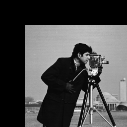
Figure 1-1: Translation

Figure 1-2: Scaling

Figure 1-3: Rotation

We’ve now covered the basic transformations. Before diving into projective transformations, it's important to first understand homogeneous coordinates, which involve adding an extra dimension to regular Cartesian coordinates. This additional coordinate allows us to represent transformations—like translation and perspective—that aren't possible with standard 2D vectors alone.

For example, a 2D point becomes a 3D vector in homogeneous coordinates, as shown below:

$$(x,y) \rightarrow (wx,wy,w), \space w \ne 0$$

To get back to Cartesion coordinate:

$$(x', y', w) \rightarrow (\dfrac{x'}{w}, \dfrac{y'}{w})$$

• $w=1$: regular affine space
• $w=0$: point at infinity, used in projective geometry

The reason we use this form is that affine transformations—such as translation—cannot be represented using simple matrix-vector multiplication in regular Cartesian coordinates. However, they can be expressed this way using homogeneous coordinates.

Mathematically, both generic affine and projective transformations can be defined as follows:

Affine Transform

$$\begin{bmatrix} x' \\ y' \\ 1 \end{bmatrix} = \begin{bmatrix} a & b & e \\ c & d & f \\ 0 & 0 & 1 \end{bmatrix} \begin{bmatrix} x \\ y \\ 1 \end{bmatrix}$$

Projective Transform

$$\begin{bmatrix} x' \\ y' \\ 1 \end{bmatrix} = \begin{bmatrix} a & b & c \\ d & e & f \\ p & q & r \end{bmatrix} \begin{bmatrix} x \\ y \\ 1 \end{bmatrix}$$

From the matrix above, it’s clear that we can construct a 3×3 transformation matrix by adjusting the values at specific positions to achieve the desired effect. To demonstrate the power of projective transformations, we'll take a specific image, extract a portion of it, and apply a transformation that makes it appear front-facing—effectively projecting it onto a 2D plane.

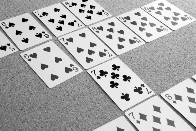
Figure 2-1: Original

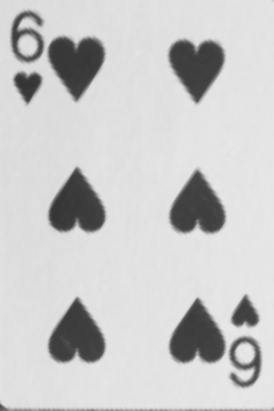
Figure 2-2: Card6

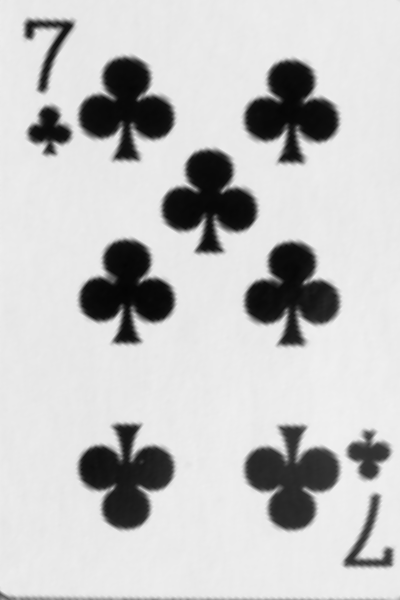
Figure 2-3: Card7

The code is provided as follows:

void kernel_callback_projective_transform(
    char **argv, const char *filename,
    void (*func)(Image *, Image *, double mat[3][3])) 
  {
  // Card 6
  double mat6[3][3] = {{2.20e-1, 1.11e-1, 5.50e1},
                       {-8.22e-2, 1.10e-1, 1.47e2},
                       {9.10e-5, -1.37e-4, 8.20e-1}};

  // Card 7
  double mat7[3][3] = {{2.21e-1, 9.12e-2, 2.20e2},
                       {-6.98e-2, 1.14e-1, 1.79e2},
                       {8.99e-5, -1.46e-4, 7.70e-1}};

  Image *img1 = new Image();
  img1->read(argv[1]);

  int W = img1->getWidth();
  int H = img1->getHeight();
  int C = img1->getCH();

  Image *img2 = new Image();
  img2->init(400, 600, 1);

  func(img1, img2, mat6);

  img2->save(filename);

  delete img1;
  delete img2;
}

void projective_transform(
    Image *in, 
    Image *out, 
    double mat[3][3]) {
  int out_W = out->getWidth();  // Use OUTPUT image dimensions
  int out_H = out->getHeight(); // Use OUTPUT image dimensions

  for (int y = 0; y < out_H; ++y) {   // Process ALL output rows
    for (int x = 0; x < out_W; ++x) { // Process ALL output columns
      double xx = mat[0][0] * x + mat[0][1] * y + mat[0][2];
      double yy = mat[1][0] * x + mat[1][1] * y + mat[1][2];
      double ss = mat[2][0] * x + mat[2][1] * y + mat[2][2];

      if (ss != 0) {
        xx /= ss;
        yy /= ss;
      }

      int value = bilinear_interpolation(in, xx, yy);
      out->set(x, y, value);
    }
  }
}

However, deriving the homography matrix involves uncovering many underlying complexities. This process lies at the heart of projective geometry and homography estimation.

A homography captures the essence of a projective transformation—including translation, rotation, scaling, and perspective distortion—between two planes or image mappings.

In short, to compute the homography matrix, we need at least four point correspondences between the input image and the target plane (typically rectified or front-facing). We may explore this further in a separate post dedicated to homography estimation.

Codebase

Conclusion

Linear algebra is no longer just an abstract concept—it has become a practical tool we can directly apply and understand in real-world scenarios. It's also a commonly used technique in computer vision, particularly for reducing overfitting and improving model performance. We're excited to explore more interesting applications in the near future.