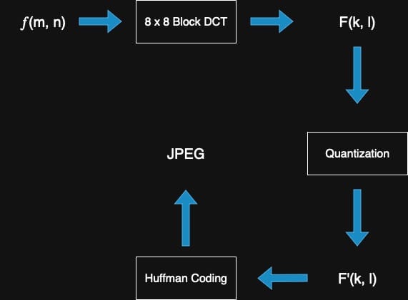
Image Compression - JPEG(II)

We previously discussed how DCT works to achieve compression in Image Compression - JPEG(I). Today, we’ll focus on quantization, which controls the trade-off between image quality and bitrate. Simply put, quantization determines how much information we choose to retain. Note that quantization is applied immediately after transforming the image from the spatial domain to the frequency domain—that is, right after the DCT step.
Quantization
Here is the formal definition of quantization:
$$Q_{i,j} \vcentcolon = \hat{F}(k,l) = round(\dfrac{F(k,l)}{q \cdot QTable(k, l)})$$
- Larger $q$ → low quality and bitrate
- Smaller $q$ → high quality and bitrate
One commonly used quantization matrix is based on an empirical design developed by the JPEG committee.
$$\begin{bmatrix} 16 & 11 & 10 & 16 & 24 & 40 & 51 & 61 \\ 12 & 12 & 14 & 19 & 26 & 58 & 60 & 55 \\ 14 & 13 & 16 & 24 & 40 & 57 & 69 & 56 \\ 14 & 17 & 22 & 29 & 51 & 87 & 80 & 62 \\ 18 & 22 & 37 & 56 & 68 &109 &103 & 77 \\ 24 & 35 & 55 & 64 & 81 &104 &113 & 92 \\ 49 & 64 & 78 & 87 &103 &121 &120 &101 \\ 72 & 92 & 95 & 98 &112 &100 &103 & 99 \end{bmatrix}$$
From the formula and matrix above, you can see that high-frequency components are divided by larger values, often resulting in zeros. In contrast, low-frequency components are preserved more accurately. This means that the Q-value directly controls how much information is retained during compression. Now, let's take a look at how this process works in practice.
Obviously, even though the DCT is invertible, the quantization step is lossy—meaning that the original data cannot be fully recovered after compression. This is why JPEG is typically referred to as a lossy (or destructive) compression technique. Now, let's take a look at the implementation.
void dct_quantize(Image *in, Image *out, int q) {
  printf("Starting DCT Quantization and Reconstruction (q=%d)...\n", q);

  in->divide(8);
  int total_blocks = in->getBlockCountX(8) * in->getBlockCountY(8);
  int processed_blocks = 0;

  for (int block_y = 0; block_y < in->getBlockCountY(8); ++block_y) {
    for (int block_x = 0; block_x < in->getBlockCountX(8); ++block_x) {
      Image block;
      in->getBlock(block_x, block_y, 8, block);

      double input_block[8][8];
      double dct_coeffs[8][8];
      double quantized_coeffs[8][8];
      double reconstructed_block[8][8];

      for (int y = 0; y < 8; ++y) {
        for (int x = 0; x < 8; ++x) {
          if (x < block.getWidth() && y < block.getHeight()) {
            if (block.getCH() == 1) {
              input_block[y][x] = block.get(x, y) - 128.0;
            } else {
              for (int c = 0; c < block.getCH(); ++c) {
                input_block[y][x] = block.get(x, y, c) - 128.0;
              }
            }
          } else {
            input_block[y][x] = 0.0;
          }
        }
      }

      DCT8x8(input_block, dct_coeffs);

      // Quantization: divide by (QTable * q), round, then multiply back
      for (int y = 0; y < 8; ++y) {
        for (int x = 0; x < 8; ++x) {
          double qtable_val = QTable[y][x] * q;
          quantized_coeffs[y][x] =
              round(dct_coeffs[y][x] / qtable_val) * qtable_val;
        }
      }

      IDCT8x8(quantized_coeffs, reconstructed_block);

      // Create reconstructed block and add back 128
      Image restored_block;
      restored_block.init(
        block.getWidth(),
        block.getHeight(),
        block.getCH());

      for (int y = 0; y < block.getHeight(); ++y) {
        for (int x = 0; x < block.getWidth(); ++x) {
          if (block.getCH() == 1) {
            restored_block.set(x, y, reconstructed_block[y][x] + 128.0);
          } else {
            for (int c = 0; c < block.getCH(); ++c) {
              restored_block.set(
                x, y, c, reconstructed_block[y][x] + 128.0);
            }
          }
        }
      }

      out->setBlock(block_x, block_y, 8, restored_block);

      ++processed_blocks;
      if (processed_blocks % 100 == 0) {
        printf("Processed %d/%d blocks\n", processed_blocks, total_blocks);
      }
    }
  }

  printf("\n=== DCT Quantization and Reconstruction Complete ===\n");
  printf("✓ Quantization factor (q): %d\n", q);
  printf("✓ Applied DCT → Quantization → IDCT to all blocks\n");
  printf("✓ Reconstructed image saved. \n");
}
Quantization - CSY
I tested with Q=[5,10,25] to observe how different Q values affect the visual appearance of the images.
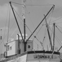
Figure 1-1: Original

Figure 1-2: Q=5
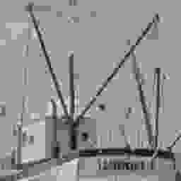
Figure 1-3: Q=15
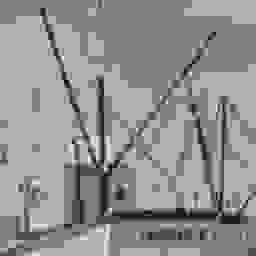
Figure 1-4: Q=25
Amazing—it's straightforward to see the impact of applying such operations. The next step is to reconstruct the image from the compressed data, which is essentially in JPEG format.
Now, it's time to visualize the trade-off between compression ratio and image quality (measured by PSNR: Peak Signal-to-Noise Ratio). This relationship can be illustrated with a trade-off curve, and the PSNR is defined by the following formula:
$$MSE = \dfrac{\sum_{x,y}(f(x,y) - g(x,y))^2}{\sum_{x,y} 1}$$
$$PSNR = 10 \cdot \log_{10}(\dfrac{255^2}{MSE})$$ [dB]
For the same image, we iterate over multiple q values and calculate the PSNR and the number of surviving (non-zero) coefficients for each.
double calculate_psnr(Image *original, Image *reconstructed) {
  int W = original->getWidth();
  int H = original->getHeight();
  int C = original->getCH();

  double mse = 0.0;
  int total_pixels = W * H * C;

  for (int y = 0; y < H; ++y) {
    for (int x = 0; x < W; ++x) {
      if (C == 1) {
        double diff = original->get(x, y) - reconstructed->get(x, y);
        mse += diff * diff;
      } else {
        for (int ch = 0; ch < C; ch++) {
          double diff = original->get(x, y, ch) \
            - reconstructed->get(x, y, ch);
          mse += diff * diff;
        }
      }
    }
  }

  mse /= total_pixels;

  if (mse == 0) {
    return 100.0;
  }

  double psnr = 10.0 * log10((255.0 * 255.0) / mse);
  return psnr;
}
PSNR Calculation - CSY
The PSNR calculation is straightforward. Now, we also implement the analysis to gain further insights.
void dct_psnr_analysis(Image *in) {
  printf(
      "Starting DCT PSNR Analysis for Quality vs Compression Trade-off...\n");

  float q_values[] = {0.05, 0.1, 0.2, 0.25, 0.5, 1,   2,   3,  4,
                      5,    6,   7,   8,    9,   10,  15,  20, 30,
                      40,   50,  75,  100,  125, 150, 175, 200};
  int num_q_values = sizeof(q_values) / sizeof(q_values[0]);

  std::string data_filename = "psnr-data.txt";
  FILE *fp = fopen(data_filename.c_str(), "w");
  if (!fp) {
    printf("Error: Could not open file %s for writing\n",
           data_filename.c_str());
    return;
  }

  fprintf(fp, "# PSNR vs Compression Trade-off Analysis\n");
  fprintf(fp, "# "
              "Q_Factor\tPSNR(dB)\tZero_Coeffs(%)\tCompression_"
              "Ratio\tRetention_Ratio\tEnergy_"
              "Retention(%)\n");

  printf("\n=== PSNR vs Compression Analysis ===\n");
  printf("Q\tPSNR(dB)\tZero(%)\tCompress\t\tEnergy(%)\n");
  printf("----\t--------\t------\t-----------\t\t---------\n");

  for (int i = 0; i < num_q_values; ++i) {
    float q = q_values[i];

    Image *reconstructed = new Image();
    reconstructed->init(in->getWidth(), in->getHeight(), in->getCH());

    in->divide(8);

    double total_original_energy = 0.0;
    double total_quantized_energy = 0.0;
    int zero_coeffs = 0;
    int total_coeffs = 0;

    for (int block_y = 0; block_y < in->getBlockCountY(8); ++block_y) {
      for (int block_x = 0; block_x < in->getBlockCountX(8); ++block_x) {
        Image block;
        in->getBlock(block_x, block_y, 8, block);

        double input_block[8][8];
        double dct_coeffs[8][8];
        double quantized_coeffs[8][8];
        double reconstructed_block[8][8];

        for (int y = 0; y < 8; ++y) {
          for (int x = 0; x < 8; ++x) {
            if (x < block.getWidth() && y < block.getHeight()) {
              if (block.getCH() == 1) {
                input_block[y][x] = block.get(x, y) - 128.0;
              } else {
                input_block[y][x] = block.get(x, y, 0) - 128.0;
              }
            } else {
              input_block[y][x] = 0.0;
            }
          }
        }

        DCT8x8(input_block, dct_coeffs);

        for (int y = 0; y < 8; ++y) {
          for (int x = 0; x < 8; ++x) {
            double quantization_step = QTable[y][x] * q;
            double original_coeff = dct_coeffs[y][x];
            double quantized_coeff =
                round(original_coeff / quantization_step) \
                * quantization_step;

            quantized_coeffs[y][x] = quantized_coeff;

            total_original_energy += original_coeff * original_coeff;
            total_quantized_energy += quantized_coeff * quantized_coeff;
            ++total_coeffs;

            if (abs(round(original_coeff / quantization_step)) == 0) {
              zero_coeffs++;
            }
          }
        }

        IDCT8x8(quantized_coeffs, reconstructed_block);

        Image restored_block;
        restored_block.init(
          block.getWidth(), block.getHeight(), block.getCH());

        for (int y = 0; y < block.getHeight(); ++y) {
          for (int x = 0; x < block.getWidth(); ++x) {
            double pixel_value = reconstructed_block[y][x] + 128.0;
            pixel_value = fmax(0, fmin(255, pixel_value));

            if (block.getCH() == 1) {
              restored_block.set(x, y, pixel_value);
            } else {
              for (int ch = 0; ch < block.getCH(); ++ch) {
                restored_block.set(x, y, ch, pixel_value);
              }
            }
          }
        }

        reconstructed->setBlock(block_x, block_y, 8, restored_block);
      }
    }

    double psnr = calculate_psnr(in, reconstructed);

    double zero_percentage = (double)zero_coeffs / total_coeffs * 100.0;
    double compression_ratio =
        (double)zero_coeffs / (in->getHeight() * in->getWidth() \
          * in->getCH());
    double retention_ratio =
        (double)(total_coeffs - zero_coeffs) / total_coeffs;
    double energy_retention =
        total_quantized_energy / total_original_energy * 100.0;

    printf("%d\t%.4f\t\t%.4f\t%.4fx(%.1f%%)\t%.4f\t%.4f\n", q, psnr,
           zero_percentage, compression_ratio, retention_ratio * 100,
           energy_retention);

    fprintf(fp, "%d\t%.4f\t%.4f\t%.4f\t%.4f\t%.4f\n", q, psnr, zero_percentage,
            compression_ratio, retention_ratio, energy_retention);

    delete reconstructed;
  }

  fclose(fp);

  printf("\n=== PSNR Analysis Complete ===\n");
  printf("✓ Trade-off data saved to: %s\n", data_filename.c_str());
  printf("✓ Use this data to plot PSNR vs Compression curve\n");

  printf("\n💡 Key Findings:\n");
  printf("• Q=1: Highest quality (PSNR), lowest compression\n");
  printf("• Q=10-20: Good balance for most applications\n");
  printf("• Q=50+: High compression but visible quality loss\n");
  printf("• Zero coefficients indicate compression potential\n");
}
PSNR Analysis - CSY
We start by passing in an image in PGM format. Then, we iterate over multiple q values, calculating the PSNR and the ratio of surviving coefficients for each. Finally, we use a script to generate the diagram shown below.
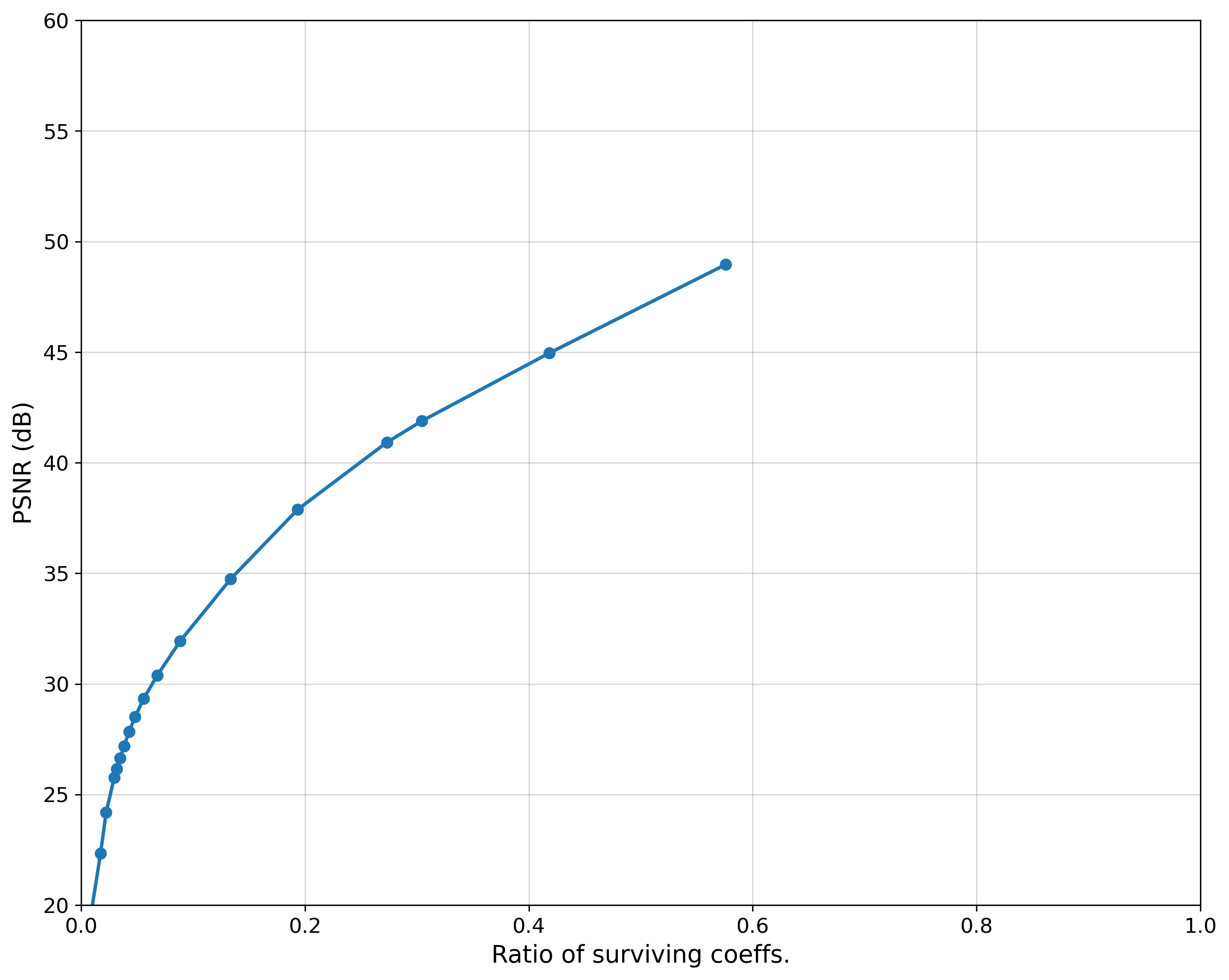
As you can see, a higher PSNR corresponds to a higher ratio of surviving coefficients. This indicates better image quality, as more information from the original image is preserved.
Conclusion
Whew, that was a long topic! But with this post and the previous one on JPEG, we’ve gained a solid understanding of how compression works in everyday life and its wide range of applications.
What’s fascinating is that the core idea behind compression isn’t limited to images—you can apply similar principles to reinforcement learning trajectories or other types of data with shared characteristics. With this, we now have one more powerful tool in our arsenal.


