Image Filter and Edge Detection

Yesterday, we discussed Luminance Inversion and Color Swapping as our starting points in image processing. Today, let's explore what edge detection is and how it is used.

Mean Filter (aka. Kernel)

Why do we apply this filter to images? Here are a few reasons:

• Noise Reduction: Removes random noise and reduces abrupt intensity variations, helping to clean up the image for further processing.
• Smoothing: Softens the image before applying edge detection to minimize false edges caused by minor fluctuations or texture details.

Simply put, the mean filter is commonly used as a preprocessing step before edge detection to reduce sharp intensity variations—sudden changes in signal strength or pixel values across an image. The following snippet illustrates how it works internally and you can find codebase here:

void mean_filter(Image *in, Image *out, const int winsize) {
  int W = in->getWidth();
  int H = in->getHeight();
  int C = in->getCH();

  for (int y = 0; y < H; ++y) {
    for (int x = 0; x < W; ++x) {
      int cnt = 0;
      double mean_out = 0;

      for (int j = -winsize; j <= winsize; ++j) {
        int yp = y + j;

        if (yp < 0)
          yp = yp + H;
        if (yp > H - 1)
          yp = yp - H;

        for (int i = -winsize; i <= winsize; ++i) {
          int xp = x + i;
          if (xp < 0)
            xp = xp + W;
          if (xp > W - 1)
            xp = xp - W;

          double val_in = in->get(xp, yp);
          mean_out += val_in;
          ++cnt;
        }
      }

      mean_out = (double)mean_out / (double)cnt;
      out->set(x, y, mean_out);
    }
  }
}

But why does the mean filter blur an image?

Take this 1D pixel array as an example: [10, 10, 10, 10, 200, 10, 10]. If we apply a mean filter with a window size of 3, the result becomes approximately [10, 10, 10, 73.3, 73.3, 73.3]. This shows that the sharp spike (the value 200) is smoothed out, but the contrast is also significantly reduced.

We can also understand this from the perspective of the Fourier Transform, which converts an image from the spatial domain to the frequency domain. In this context, we can interpret frequency as follows:

• Low Frequency: smooth areas or gradual changes
• High Frequency: sharp edges or sudden intensity changes.

Therefore, the mean filter is essentially a type of low-pass filter—it allows low-frequency components to pass through while blocking or reducing high-frequency information.

From the frequency domain perspective, applying a mean filter is equivalent to convolving the image with a box kernel in the spatial domain.

In short, when we apply a mean filter, we suppress high-frequency components—and this suppression is what we perceive as blurring.

Edge Detection

Edge detection is a technique used to identify boundaries or edges in an image, where there are sharp intensity variations (gradients). It serves as a counterpart to the mean filter—while the mean filter smooths out such variations, edge detection emphasizes them.

Some common edge detection methods include:

• Sobel Operator: detects edges by applying convolution with specific kernels that highlight intensity changes in the horizontal or vertical direction.
• Laplacian Operator: identifies edges by detecting zero-crossings in the second derivative of intensity values, capturing regions where the rate of change shifts sharply.

Figure 1: Original

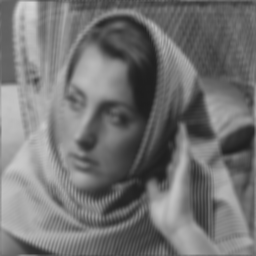
Figure 2: Mean Filter

Sobel Operator

The Sobel operator identifies edges in an image by computing the gradient of pixel intensity values. It emphasizes regions with sharp changes in brightness, which often correspond to edges.

It uses two 3×3 convolution kernels: one to detect horizontal edges and the other for vertical edges. The Sobel operator effectively combines gradient calculation and smoothing in a single step, helping reduce the impact of noise while detecting edge direction and strength.

$$Sobel_{x} = \begin{bmatrix} -1 & 0 & 1 \\ -2 & 0 & 2 \\ -1 & 0 & 1 \end{bmatrix}$$

$$Sobel_{y} = \begin{bmatrix} -1 & -2 & -1 \\ 0 & 0 & 0 \\ 1 & 2 & 1 \end{bmatrix}$$

These kernels are applied to the image by convolving them with each pixel and its neighboring pixels. The following code demonstrates this process:

const int SOBEL_HRZ_K[3][3] = {{-1, 0, 1}, {-2, 0, 2}, {-1, 0, 1}};

void horizontal_edge_filter(Image *in, Image *out, const int winsize) {
  int W = in->getWidth();
  int H = in->getHeight();
  int C = in->getCH();

  for (int y = 0; y < H; ++y) {
    for (int x = 0; x < W; ++x) {
      double sobel_hrz_val = 0.0;

      for (int j = -winsize; j <= winsize; ++j) {
        int yp = y + j;
        if (yp < 0)
          yp = yp + H;
        if (yp > H - 1)
          yp = yp - H;

        for (int i = -winsize; i <= winsize; ++i) {
          int xp = x + i;
          if (xp < 0)
            xp = xp + W;
          if (xp > W - 1)
            xp = xp - W;

          double val_in = in->get(xp, yp);
          sobel_hrz_val += val_in * SOBEL_HRZ_K[j + 1][i + 1];
        }
      }

      sobel_hrz_val = std::max(0.0, std::min(255.0, sobel_hrz_val + 128.0));
      out->set(x, y, sobel_hrz_val);
    }
  }
}

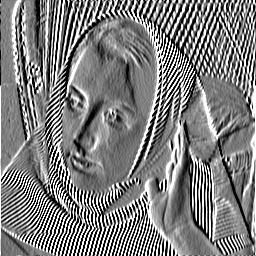
Figure 3: Horizontal

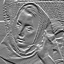
Figure 4: Vertical

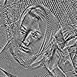
Figure 5: Hrz-Vrt

From the images, we can see how edges are detected in both horizontal and vertical directions. Next, let me introduce another important operator called the Laplacian operator.

In this example, I first applied horizontal edge detection followed by vertical edge detection, which produces some interesting results.

Laplacian Operator

The Laplacian operator measures how much a pixel’s value differs from its neighbors, effectively highlighting areas of rapid intensity change—such as edges.

Mathematically, the Laplacian operator is defined as:

$$\nabla^2f = \dfrac{\partial^2f}{\partial x^2} + \dfrac{\partial^2f}{\partial y^2}$$

There are two commonly used Laplacian kernels: one that includes diagonal neighbors and one that does not. They are as follows:

$$L = \begin{bmatrix} 0 & 1 & 0 \\ 1 & -4 & 1 \\ 0 & 1 & 0 \end{bmatrix}, L_{diag} = \begin{bmatrix} 1 & 1 & 1 \\ 1 & 8 & 1 \\ 1 & 1 & 1 \end{bmatrix}$$

While the Laplacian operator captures features in all directions, it is more sensitive to noise. Because it involves the second derivative, which treats all directions equally, even small noise fluctuations can have a large impact on the result.

The code snippet is provided below:

const int LAPLACIAN_K[3][3] = {{0, 1, 0}, {1, -4, 1}, {0, 1, 0}};
const int LAPLACIAN_K_DIAG[3][3] = {{1, 1, 1}, {1, -8, 1}, {1, 1, 1}};

void laplacian_filter(Image *in, Image *out, const int winsize) {
  int W = in->getWidth();
  int H = in->getHeight();
  int C = in->getCH();

  for (int y = 0; y < H; ++y) {
    for (int x = 0; x < W; ++x) {
      double lap_val = 0.0;

      for (int j = -winsize; j <= winsize; ++j) {
        int yp = y + j;
        if (yp < 0)
          yp = 0;
        if (yp > H - 1)
          yp = H - 1;

        for (int i = -winsize; i <= winsize; ++i) {
          int xp = x + i;
          if (xp < 0)
            xp = 0;
          if (xp > W - 1)
            xp = W - 1;

          double val_in = in->get(xp, yp);
          lap_val += val_in * LAPLACIAN_K_DIAG[j + 1][i + 1];
        }
      }

      lap_val = std::max(0.0, std::min(255.0, lap_val));
      out->set(x, y, lap_val);
    }
  }
}

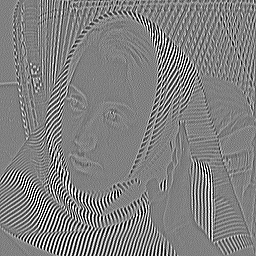
Figure 6: Laplacian

There is one more topic I’d like to discuss: Detail Enhancement, which is used to clarify and sharpen textures in an image. Some common methods include:

1. Unsharp Masking (USM): enhances edges and fine details by adding a scaled difference between the original image and its blurred version

$$\text{Enhanced} = \text{Original} + \alpha \cdot (\text{Original} - \text{Blurred})$$

2. Bilateral Filtering: eparates the image into base and detail layers while smoothing, preserving edges by considering both spatial closeness and intensity similarity
3. Laplacian of Gaussian(LoG): Enhances details by combining Gaussian smoothing with the Laplacian operator to detect regions of rapid intensity change.

Here, we only apply one method: Unsharp Masking (USM).

void enhance_mean_filter(Image *in, Image *out, const int winsize) {
  int W = in->getWidth();
  int H = in->getHeight();
  int C = in->getCH();

  for (int y = 0; y < H; ++y) {
    for (int x = 0; x < W; ++x) {
      int count = 0;
      double mean_out = 0.0;

      for (int j = -winsize; j <= winsize; ++j) {
        int yp = y + j;
        if (yp < 0)
          yp = 0;
        if (yp > H - 1)
          yp = H - 1;

        for (int i = -winsize; i <= winsize; ++i) {
          int xp = x + i;
          if (xp < 0)
            xp = 0;
          if (xp > W - 1)
            xp = W - 1;

          double val_in = in->get(xp, yp);
          mean_out += val_in;
          count++;
        }
      }

      mean_out = mean_out / (double)count;
      double origin_val = in->get(x, y);
      double val_out = origin_val + (origin_val - mean_out);

      val_out = std::max(0.0, std::min(255.0, val_out + 128.0));
      out->set(x, y, val_out);
    }
  }
}

Figure 7: Laplacian

Conclusion

Whew, we’ve applied several kernels to the same image and can clearly see how each one alters the result. These filters are very useful for extracting specific features from images and can be further applied to tasks like image classification, helping to reduce overfitting and improve model performance.

That said, there are still many more kernels to explore, and it’s the underlying mathematical foundations that truly fascinate me.