MDP(Markov Decision Process)

Today, let's talk about the foundation stone of RL. You can refer to this to grasp basic understanding of RL.
Introduction to MDP
Markov Decision Process (MDP) is the fundamental of RL, and is introduced in Reinforcement Learning: An Introduction at Chapter 3 of the book. So, what MDP really is? An image worths thousand of words.
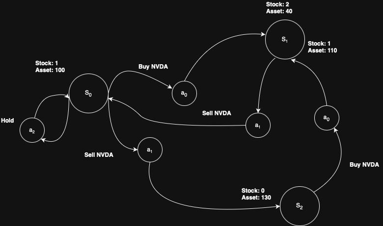
The above image depicts the MDP inner work even though it is not strict enough. However, what does this really indicates? MDP is nothing more than a mathematical framework which guides us modeling the decision-making procedure. The core components of MDP are listed as below:
- State(S): a finite set of possible situations an agent can be in.
- Action(A): a finite set of choices an agent can take.
- Reward Function(R): immediate reward an agent receives.
- Transition Model(P): the probability of moving from one state(s) to next state(s')
- Discount Factor(γ-gamma): a value between 0 and 1 that controls the importance of future rewards.
- γ close to 0 means short-sighted
- γ close to 1 means far-sighted
As you can see, the components of MDP are alike to RL. Or, one can declare RL derives from MDP concept.
How MDP Work: Goal and Policy
MDP can be easily described as the following.
Goal: the primary goal in an MDP is to find an optimal policy.
Policy(π): a strategy that tells the agent what action to take in each state. Think this as an image mapping which makes state to actions ($π(s) → a$).
- Deterministic Policy: always prescribes the same action.
- Stochastic Policy: a probability distribution over possible actions.
Optimal Policy($π^{*}$): policy that maximizes the expected cumulative discounted reward over time.
A formal expression is defined as below.
Transition Probability: $p(s'|s,a) = Pr[s_{t+1}=s'|S_t=s,A_t=a]$
Reward Function: $r(s,a,s') = E[R_{t+1}|S_t=s,A_t=a,S_{t+1}=s']$
However, in RL, we typically focus on long-term rewards rather than immediate rewards from individual actions. As a result, policies in Markov Decision Processes (MDPs) are defined to maximize the cumulative reward, also known as the discounted reward sum. This objective is framed as an optimization problem.
Cumulative Reward: $G_t = R_{t+1} + γR_{t+2} + γ^2R_{t+3} + \cdots = \sum_{t=1}^∞ γ^{k-1}R_{t+k}$
Value(Target) Function: $v_π(s) = E_π[G_t|S_t=s]$
The subscript π on the expectation E indicates the policy currently being followed (i.e., a probability distribution over actions). The goal is, of course, to find the optimal policy that yields the maximum possible reward — analogous to someone trying to maximize profit in the financial market.
Bellman Equation
So far, we have discussed the backbone of RL, and its detailed components of itself. Let's dive into the Bellman Equation which rewrites the calculation of value function into a recursive form. We derive the equation as below.
$$G_t = R_{t+1} + γR_{t+2} + γ^2R_{t+3} + \cdots = \sum_{t=1}^∞ γ^{k-1}R_{t+k}$$
$$G_t = R_{t+1} + γG_{t+1}$$
Given the value function,
$E_π[G_t|S_t=s] = E_π[R_{t+1}|S_t=s] + γE_π[G_{t+1}|S_t=s]$
The first term on the right-hand side depends only on the state s; however, the reward function above depends on both the action and the next state. Therefore, we need to multiply by the marginal probability and incorporate it back into the original function.
$$E_π[R_{t+1}|S_t=s] = \sum_aπ(a|s)\sum_{s'}p(s'|s,a)r(s,a,r')$$
The second term of right side is similar to the first term, in which we rewrite as below.
$$γE_π[G_{t+1}|S_t=s] = γ\sum_aπ(a|s)\sum_{s'}p(s'|s,a)v_π(s')$$
Combined those two terms, the equation could be deduced as below.
$$v_π(s) = \sum_aπ(a|s)\sum_{s'}p(s'|s,a)[r(s,a,s')+γv_π(s')]$$
For the action-value function, we only need to consider a specific action in a given state. Therefore, the action-value function and the value function form a complementary (or dual) relationship.
$$v_π(s) = \sum_aπ(a|s)q_π(s)$$
$$q_π(s) = \sum_{s'}p(s'|s,a)[r(s,a,s')+γv_π(s')] \equiv E_π[G_t|S_t=s,A_t=a]$$
Besides, the optimal value and action-value function are expressed with *.
$$v_*(s) = \max_πv_π(s)$$
$$q_*(s,a) = \max_πq_π(s,a)$$
Whew, that was quite a long discussion — but the journey is just beginning. Next time, we’ll explore how to handle dynamic planning using the Bellman Equation, diving into value iteration and policy iteration with some code snippets.


