Monte Carlo

In previous posts, we discussed the Bellman Equation in the context of Bellman Equation - Policy Iteration and Bellman Equation - Value Iteration, both of which assume access to background knowledge about the model—specifically, the transition and reward functions. However, in most real-world problems, we don’t have prior information about the environment. This scenario is referred to as Model-Free. We previously highlighted the differences between Model-Based and Model-Free approaches in our discussion on Bellman Equation - Policy Iteration.
When the environment is unknown, we need a method to gather data through interaction—and that’s where learning by doing comes in. Just like how humans learn to ride a bike, we don’t teach kids by giving them lectures on physics, balance, or gyroscopic forces. Instead, they get on the bike, start pedaling, and wobble their way through the experience until they learn to balance. This trial-and-error process is fundamental to Reinforcement Learning (RL), as you’ll see in the sections that follow.
Monte Carlo Introduction
So, what is the Monte Carlo (MC) method?
Monte Carlo methods are a class of model-free algorithms that learn optimal actions by averaging the outcomes of many simulated experiences. Imagine you're playing a maze game and trying to find the way out. You would run through the maze multiple times, trying different paths at random. For each attempt, you'd track whether the path leads to an exit and how long it takes. Over time, by averaging the results of these trials, you can estimate which actions are more likely to lead to success.
The first time I heard about Monte Carlo methods was during a probability and statistics lecture from MIT. I found it quite profound to learn that this method could be used to estimate the value of π through a simple yet vivid experiment.
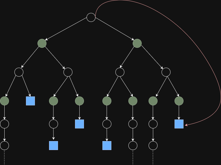
As you could see from the diagram, Monte Carlo usually evaluates its actions through one full episode (e.g, terminal state reached). To average returns from episodes, there are two commonly used approaches to do within one episode itself:
- First-Visit MC: only use the first visit to state s in an episode
- Pros: reduce bias
- Cons: slower convergence and more variance
- Every-Visit MC: use every visit to state s in an episode
- Pros: reduce variance and faster convergence
- Cons: more bias
Also, based on the diagram, we could define the recursive formula:
$$V_{t+1}(s) = V_{t}(s) + \alpha_t(G_t - V_{t}(S_t))$$
Besides, the convergence can be guaranteed with Robbins-Monro condition:
$$\sum_{t=0}^{∞}⍺_{t} = ∞$$
$$\sum_{t=0}^{∞} (⍺_{t})^{2} < +∞$$
Monte Carlo Implementation
Here, we will use Blackjack to show how MC works internally.
import numpy as np
from collections import defaultdict

class BlackjackMC:
    def __init__(self):
        self.deck = self._create_deck()
        self.action_values = defaultdict(lambda: {'hit': 0, 'stand': 0})
        self.action_counts = defaultdict(lambda: {'hit': 0, 'stand': 0})

    def _create_deck(self):
        """Create a deck of cards (1-10, with face cards as 10)"""
        return list(range(1, 11)) * 4  # 4 suits

    def _draw_card(self):
        """Draw a random card from the deck"""
        return np.random.choice(self.deck)

    def _get_hand_value(self, hand):
        """Calculate the value of a hand, handling aces (1 or 11)"""
        value = sum(hand)
        if 1 in hand and value + 10 <= 21:
            value += 10
        return value

    def _is_bust(self, hand):
        """Check if a hand is bust (over 21)"""
        return self._get_hand_value(hand) > 21

    def _dealer_play(self, dealer_hand):
        """Dealer plays according to standard rules (hit on 16 or less)"""
        while self._get_hand_value(dealer_hand) < 17:
            dealer_hand.append(self._draw_card())
        return dealer_hand

    def _get_state(self, player_hand, dealer_card):
        """Get the current state of the game"""
        return (self._get_hand_value(player_hand), dealer_card)

    def play_episode(self):
        """Play one episode of blackjack"""

        player_hand = [self._draw_card(), self._draw_card()]
        dealer_hand = [self._draw_card(), self._draw_card()]
        dealer_card = dealer_hand[0]  # Only one dealer card is visible

        states = []
        actions = []
        rewards = []

        while True:
            # Player's turn
            state = self._get_state(player_hand, dealer_card)
            states.append(state)

            # Choose action (hit or stand) based on current estimates
            if self.action_counts[state]['hit'] == 0 and \
               self.action_counts[state]['stand'] == 0:
                action = np.random.choice(['hit', 'stand'])
            else:
                hit_value = self.action_values[state]['hit'] \
                    / max(1, self.action_counts[state]['hit'])
                stand_value = self.action_values[state]['stand'] \
                    / max(1, self.action_counts[state]['stand'])
                action = 'hit' if hit_value > stand_value else 'stand'

            actions.append(action)

            if action == 'hit':
                player_hand.append(self._draw_card())
                if self._is_bust(player_hand):
                    rewards.append(-1) # Player loses
                    break
            else:
                # Dealer's turn
                dealer_hand = self._dealer_play(dealer_hand)
                dealer_value = self._get_hand_value(dealer_hand)
                player_value = self._get_hand_value(player_hand)

                if self._is_bust(dealer_hand):
                    rewards.append(1)  # Dealer busts, player wins
                elif dealer_value > player_value:
                    rewards.append(-1)  # Dealer wins
                elif dealer_value < player_value:
                    rewards.append(1)  # Player wins
                else:
                    rewards.append(0)  # Draw
                break

        # Update action values using Monte Carlo method
        for i, (state, action) in enumerate(zip(states, actions)):
            # Calculate return (sum of rewards from this point)
            G = sum(rewards[i:])
            self.action_values[state][action] += G
            self.action_counts[state][action] += 1

    def get_policy(self):
        """Get the current policy (best action for each state)"""
        policy = {}
        for state in self.action_values:
            hit_value = self.action_values[state]['hit'] \
                / max(1, self.action_counts[state]['hit'])
            stand_value = self.action_values[state]['stand'] \
                / max(1, self.action_counts[state]['stand'])
            policy[state] = 'hit' if hit_value > stand_value else 'stand'
        return policy


def main():
    n_episodes = 10000
    agent = BlackjackMC()

    print("Training the agent...")
    for i in range(n_episodes):
        agent.play_episode()
        if (i + 1) % 1000 == 0:
            print(f"Completed {i + 1} episodes")

    policy = agent.get_policy()
    print("\nLearned Policy "
          "(Player's Hand Value, Dealer's Card) -> Action:")
    for state, action in sorted(policy.items()):
        print(f"State ({state[0]}, {state[1]}): {action}")

if __name__ == "__main__":
    main()
From the code snippet, we can observe that MC model sampling through episodes and learn the optimal policy from experience. Especially, the decision is made based on hit_value and stand_value. What's more critical is that this algorithm applies to Model-Free problems which are common in the real world.
The result should look like this which tells us based on the state, the action one should take.
State (16, 1): hit
State (16, 2): stand
State (16, 3): hit
State (16, 4): stand
State (16, 5): hit
State (16, 6): stand
State (16, 7): hit
State (16, 8): stand
State (16, 9): hit
State (16, 10): stand
State (17, 1): stand
State (17, 2): hit
State (17, 3): stand
State (17, 4): hit
State (17, 5): stand
State (17, 6): stand
State (17, 7): stand
State (17, 8): stand
State (17, 9): stand
State (17, 10): hit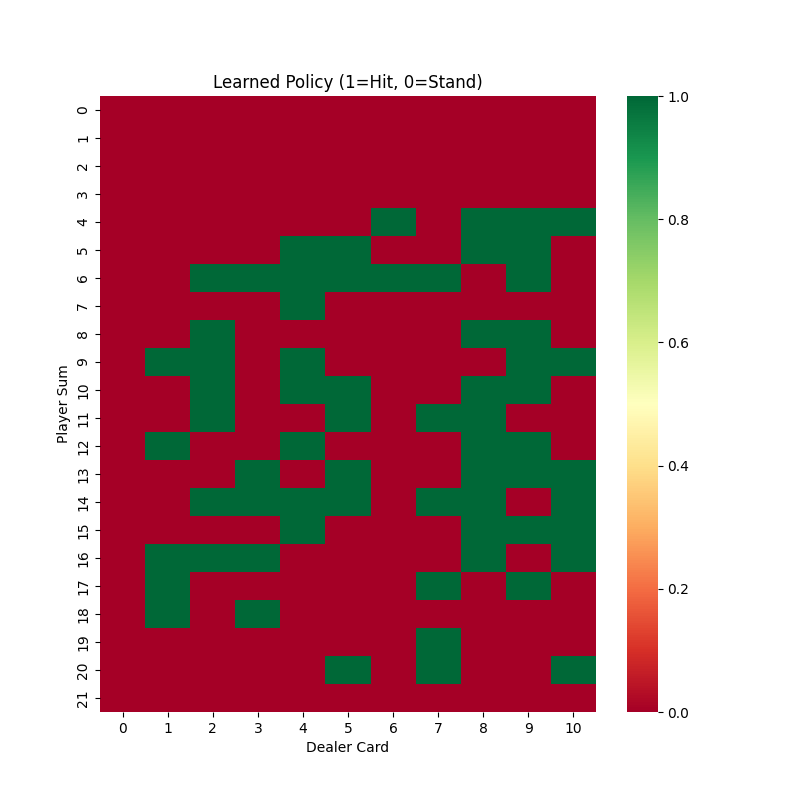
As the diagram shows, based on the states of the player and the dealer, the learned policy suggests that we should stand in most cases when the player's hand value is between 19 and 21.
Conclusion
The key strengths of MC method include simplicity, unbiased estimates, and applicability to complex, stochastic environments. However, MC methods require full episodes, can suffer from high variance, and are less suited for continuous tasks. Their reliance on real experience mirrors intuitive learning processes, making them a foundational tool in RL, with applications from games to robotics.
For deeper exploration, MC can be extended to control problems or combined with other techniques to optimize policies. We will talk about TD method in the next post, and relate these two algorithms.


