On-Off Policy

We have discussed about the difference between value-based and policy-based approaches in Value/Policy-Based Control. However, there is another important aspect to consider when distinguishing between algorithms: whether the policy is on-policy or off-policy. The definitions of these two are as follows:
- On-Policy: agent learns and improves the same policy it uses to interact with the environment
- E.g., SARSA, REINFORCE, PPO
- Off-Policy: agent learns a target policy that is different from the behavior policy used to explore the environment.
- E.g., Q-Learning, DQN, SAC
Simply put, the key difference lies in whether an algorithm uses the same policy to explore and learn from. If it does, it's called on-policy; if it uses a different policy for exploration, it's called off-policy.
- Target Policy: the policy being optimized
- Behavior Policy: the policy used for exploration
On-Off Policy Implementation
Let’s revisit the classic grid world example we used in Value/Policy-Based Control to illustrate the difference between on-policy and off-policy learning. In particular, we’ll use SARSA (an on-policy algorithm) and Q-Learning (an off-policy algorithm) to highlight how each one handles learning and exploration differently.
import numpy as np
import matplotlib.pyplot as plt

class GridWorld:
    def __init__(self, size=3):
        self.size = size
        self.state = 0
        self.goal = size * size - 1
        self.actions = [0, 1, 2, 3]
        self.n_states = size * size
        self.n_actions = len(self.actions)

    def reset(self):
        self.state = 0
        return self.state

    def step(self, action):
        row = self.state // self.size
        col = self.state % self.size

        if action == 0:  # Up
            row = max(0, row - 1)
        elif action == 1:  # Right
            col = min(self.size - 1, col + 1)
        elif action == 2:  # Down
            row = min(self.size - 1, row + 1)
        elif action == 3:  # Left
            col = max(0, col - 1)

        self.state = row * self.size + col

        done = self.state == self.goal
        reward = 1 if done else -0.1

        return self.state, reward, done

class QLearning:
    def __init__(self, n_states, n_actions,
        learning_rate=0.1,
        discount_factor=0.99,
        epsilon=0.1):
        self.q_table = np.zeros((n_states, n_actions))
        self.lr = learning_rate
        self.gamma = discount_factor
        self.epsilon = epsilon

    def choose_action(self, state):
        if np.random.random() < self.epsilon:
            return np.random.randint(0, 4)
        return np.argmax(self.q_table[state])

    def learn(self, state, action, reward, next_state):
        # Q-learning learn (off-policy)
        best_next_action = np.argmax(self.q_table[next_state])
        td_target = reward \
          + self.gamma * self.q_table[next_state][best_next_action]
        td_error = td_target - self.q_table[state][action]
        self.q_table[state][action] += self.lr * td_error

class SARSA:
    def __init__(self, n_states,
        n_actions,
        learning_rate=0.1,
        discount_factor=0.9,
        epsilon=0.1):
        self.q_table = np.zeros((n_states, n_actions))
        self.lr = learning_rate
        self.gamma = discount_factor
        self.epsilon = epsilon

    def choose_action(self, state):
        if np.random.random() < self.epsilon:
            return np.random.randint(0, 4)
        return np.argmax(self.q_table[state])

    def learn(self, state, action, reward, next_state, next_action):
        # SARSA learn (on-policy)
        td_target = reward \
          + self.gamma * self.q_table[next_state][next_action]
        td_error = td_target - self.q_table[state][action]
        self.q_table[state][action] += self.lr * td_error

def train_agent(agent, env, episodes=1000):
    rewards_history = []

    for _ in range(episodes):
        state = env.reset()
        total_reward = 0
        done = False

        # For SARSA, we need to select the initial action before the loop
        # because we need both current and next actions to update Q-values
        if isinstance(agent, SARSA):
            action = agent.choose_action(state)

        while not done:
            # For Q-learning, we can select action inside the loop
            # because we only need current state and action to update
            if isinstance(agent, QLearning):
                action = agent.choose_action(state)

            next_state, reward, done = env.step(env.actions[action])
            total_reward += reward

            if isinstance(agent, SARSA):
                # SARSA needs to know the next action to update Q-values
                # This is why it's on-policy
                #  - it uses the actual next action
                next_action = agent.choose_action(next_state)
                agent.learn(state, action, reward,
                  next_state, next_action)
                action = next_action
            else:
                # Q-learning is off-policy
                #   - it uses max Q-value of next state
                # regardless of what action will actually be taken
                agent.learn(state, action, reward, next_state)

            state = next_state

        rewards_history.append(total_reward)

    return rewards_history

def plot_results(q_learning_rewards, sarsa_rewards):
    # Calculate moving average over 10 epochs
    window_size = 10
    q_learning_avg = np.convolve(
      q_learning_rewards, np.ones(window_size)/window_size, mode='valid')
    sarsa_avg = np.convolve(
      sarsa_rewards, np.ones(window_size)/window_size, mode='valid')

    # Create figure with two subplots
    _, (ax1, ax2) = plt.subplots(2, 1, figsize=(12, 10))

    # Q-learning plot
    ax1.plot(q_learning_avg,
      label='10-epoch average', color='blue', linewidth=2)
    ax1.set_title('Q-learning Performance')
    ax1.set_xlabel('Episodes')
    ax1.set_ylabel('Total Reward')
    ax1.grid(True)
    ax1.legend()

    # SARSA plot
    ax2.plot(sarsa_avg,
      label='10-epoch average', color='orange', linewidth=2)
    ax2.set_title('SARSA Performance')
    ax2.set_xlabel('Episodes')
    ax2.set_ylabel('Total Reward')
    ax2.grid(True)
    ax2.legend()

    plt.tight_layout()
    plt.show()

def train_and_plot():
    # Create environment
    env = GridWorld(size=3)

    # Initialize agents
    q_learning_agent = QLearning(env.n_states, env.n_actions)
    sarsa_agent = SARSA(env.n_states, env.n_actions)

    # Train agents
    print("Training Q-learning agent...")
    q_learning_rewards = train_agent(q_learning_agent, env)

    print("Training SARSA agent...")
    sarsa_rewards = train_agent(sarsa_agent, env)

    # Plot results
    plot_results(q_learning_rewards, sarsa_rewards)

    # Print final Q-tables
    print("\nQ-learning final Q-table:")
    print(q_learning_agent.q_table)
    print("\nSARSA final Q-table:")
    print(sarsa_agent.q_table)

if __name__ == "__main__":
    train_and_plot()
We can observe from the QLearning and SARSA classes to know their difference in learn method. The former one always choose the action which results in maximum value, whereas SARSA always follow the action it uses to explore the environment.
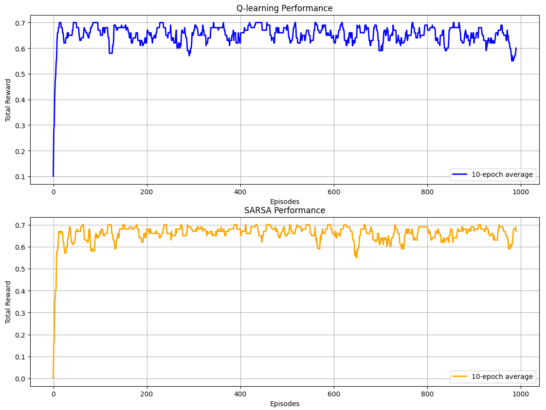
From the diagram, we can see that both algorithms perform well on the simple grid world task. However, their individual strengths become more apparent in more complex environments — something we'll explore in future examples.
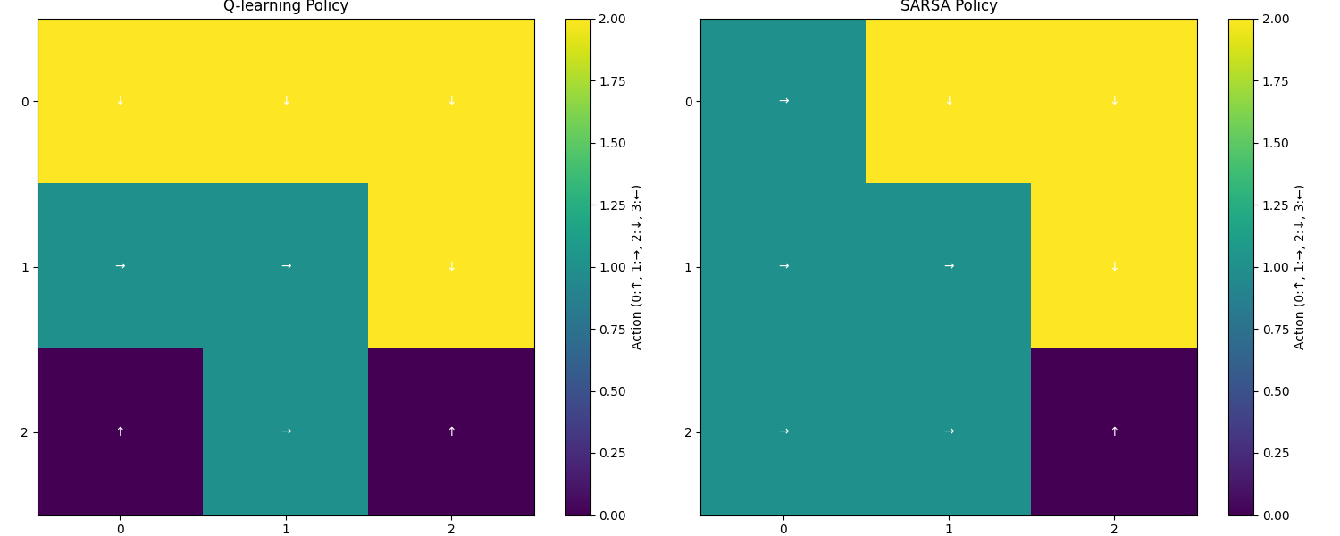
Below, we show how the final policies learned by each algorithm behave:
Conclusion
Now that we understand the difference between on-policy and off-policy learning, there’s still much more to explore — especially when it comes to their individual strengths and how we might overcome their limitations. In fact, this idea of combining the best of both worlds is exactly what motivates approaches like the Actor-Critic model, which blends policy-based and value-based methods.
Also, I haven’t gone into the details of the algorithms themselves here because I plan to explore each one more deeply in separate posts.
Over the past few days, we’ve covered the basics of reinforcement learning — but how can we actually apply it to real-world problems? That’s exactly what I’ll be focusing on next.


