Q-Learning

Today, we’re going to introduce one of the most well-known value-based reinforcement learning (RL) approaches: Q-Learning.
So, what is Q-Learning?
Q-Learning is a method where an agent learns to make decisions by estimating the value of taking certain actions in different states. It maintains a table—called a Q-table—that stores the expected future rewards for each state-action pair. As the agent explores the environment, it updates this table using feedback from its experiences, striking a balance between exploration (trying new actions) and exploitation (choosing the best-known action). This process continues until the values in the table converge.
However, Q-Learning is not suitable for environments with high-dimensional or continuous state spaces, as the Q-table becomes impractically large.
Q-Learning Introduction
A model-free RL algorithm which learns an optimal action-value function, known as the Q-function, which estimates the expected cumulative reward for taking a specific action in a given state and following a behavior policy simply for exploration thereafter. Below describes how Q-learning is defined:
$$Q(s,a) \leftarrow Q(s,a) + \alpha[r + \gamma \max_{a'}Q(s',a') - Q(s,a)]$$
where:
- $s$: current state
- $a$: action taken
- $r$: immediate reward
- $s'$: next state
- $\alpha$: learning rate
- $\gamma$: discount rate
- $\max_{a'}Q(s',a')$: maximum Q-value for the next state over all possible actions
Pros and Cons
Pros:
- Model-Free: does not require knowledge of the environment's dynamics
- Off-Policy: allows for learning from exploration using different policy
- Simplicity: easy to understand compared to policy-based methods
Cons:
- Scalability: struggles with large state spaces with Q-table (solved via neural network)
- No Generalization: lacks the ability to generalize across similar states or actions
- Exploration-Exploitation: balance can be tricky and affects performance
Q-Learning Implementation
Here, we use the good old friend example-Frozen Lake, which is provided by the Gymnasium package.
import time
import argparse
import numpy as np
import gymnasium as gym
import matplotlib.pyplot as plt

class QLearningAgent:
    def __init__(self, env,
      learning_rate=0.1,
      discount_factor=0.95,
      epsilon=1.0,
      epsilon_decay=0.999,
      epsilon_min=0.01):
        self.env = env
        self.lr = learning_rate
        self.gamma = discount_factor
        self.epsilon = epsilon
        self.epsilon_decay = epsilon_decay
        self.epsilon_min = epsilon_min

        self.q_table = np.zeros(
          (env.observation_space.n, env.action_space.n)
        )

    def _choose_action(self, state):
        if np.random.random() < self.epsilon:
            return self.env.action_space.sample()
        else:
            return np.argmax(self.q_table[state])

    def learn(self, state, action, reward, next_state, done):
        old_value = self.q_table[state, action]
        next_max = np.max(self.q_table[next_state])

        new_value = (1 - self.lr) * old_value \
          + self.lr * (reward + self.gamma * next_max * (1 - done))
        self.q_table[state, action] = new_value

        if done:
            self.epsilon = max(
              self.epsilon_min,
              self.epsilon * self.epsilon_decay
            )

    def train(self, episodes):
        rewards = []

        for e in range(1, episodes + 1):
            state, _ = self.env.reset()
            total_reward = 0
            done = False

            print(f"-------------------- Episode {e} --------------------")

            while not done:
                action = self._choose_action(state)
                next_state, reward, terminated, truncated, _ = \
                  self.env.step(action)
                done = terminated or truncated

                print(f"State: {state}, Action: {action}, Reward: {reward}, Next State: {next_state}, Done: {done}")

                self.learn(state, action, reward, next_state, done)

                state = next_state
                total_reward += reward

            rewards.append(total_reward)

            if e % 100 == 0:
                print(f"Episode {e}, Average Reward: {np.mean(rewards[-100:]):.2f}, Epsilon: {self.epsilon:.2f}")

        return rewards

    def play_episode(self):
        state, _ = self.env.reset()
        total_reward = 0
        done = False

        while not done:
            action = np.argmax(self.q_table[state])
            state, reward, terminated, truncated, _ = self.env.step(action)
            done = terminated or truncated
            total_reward += reward

            self.env.render()
            time.sleep(0.5)

        return total_reward

    def save_model(self, filename='q_table.npy'):
        np.save(filename, self.q_table)
        print(f"Model saved to {filename}")

    def load_model(self, filename='q_table.npy'):
        try:
            self.q_table = np.load(filename)
            print(f"Model loaded from {filename}")
            return True
        except FileNotFoundError:
            print(f"No saved model found at {filename}")
            return False

def plot_rewards(rewards):
    window_size = 50
    avg_rewards = []
    for i in range(0, len(rewards), window_size):
        window = rewards[i:i + window_size]
        if len(window) == window_size:
            avg_rewards.append(np.mean(window))

    plt.figure(figsize=(10, 5))
    plt.plot(range(
      window_size, len(rewards) + 1, window_size),
      avg_rewards, 'b-')
    plt.title('Average Rewards per 10 Episodes')
    plt.xlabel('Episode')
    plt.ylabel('Average Reward')
    plt.grid(True)
    plt.show()

def get_env_info(env):
    print(f"Observation space number of states: {env.observation_space.n}")
    print(f"Action space number of actions: {env.action_space.n}")

def simulate(agent, episodes=5):
    print("\nPlaying episodes with trained agent:")

    for i in range(episodes):
        print(f"\nEpisode {i+1}")
        total_reward = agent.play_episode()
        print(f"Total reward: {total_reward}")

def main(args):
    if args.render:
        env = gym.make('FrozenLake-v1', render_mode="human")
    else:
        env = gym.make('FrozenLake-v1')

    get_env_info(env)

    agent = QLearningAgent(env)

    if args.render:
        # Try to load existing model
        if not agent.load_model():
            print("No saved model found. Please train the model first.")
            return
    else:
        # Train and save the model
        rewards = agent.train(episodes=args.episodes)
        agent.save_model()
        plot_rewards(rewards)

    if args.render:
        simulate(agent, args.render_episodes)
    env.close()

if __name__ == "__main__":
    parser = argparse.ArgumentParser(description='Q-Learning DQN')
    parser.add_argument('--render',
      action='store_true', help='Render the environment')
    parser.add_argument('--episodes',
      type=int, default=1000, help='Number of episodes to simulate')
    parser.add_argument('--render_episodes',
      type=int, default=5, help='Number of episodes to render')
    parser.add_argument('--model_path',
      type=str, default='q_table.npy', help='Path to save/load the model')
    args = parser.parse_args()

    main(args)
Q-Learning - CSY
From the reward diagram, we can see that the averaged reward increases as the number of episodes grows.
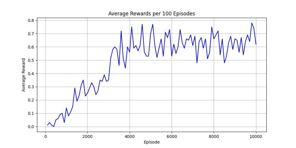
From the learning curve, we can observe that Q-learning gradually improves around episodes 3500 to 4000, but begins to oscillate afterward. This behavior suggests potential underlying issues, such as inadequate exploration, sparse rewards, or improperly tuned hyperparameters.

Conclusion
In this post, we discussed what kind of method Q-learning is — specifically, that it is a value-based and off-policy approach. We also covered its advantages and disadvantages, and implemented it on a simple grid-world environment: the Frozen Lake example.
However, as we know, Q-learning in its basic form is far from sufficient for real-world applications. In the next post, we’ll explore its more powerful successor — Deep Q Networks (DQN).


