REINFORCE

Today, we will discuss the REINFORCE algorithm (REward Increment = Nonnegative Factor × Offset Reinforcement × Characteristic Eligibility), which is derived from the Policy Gradient method we previously covered. In short, REINFORCE is a policy-based reinforcement learning algorithm that directly updates the policy—the strategy that determines which action to take in a given state.

REINFORCE Introduction

A Monte Carlo policy gradient algorithm that optimizes a parameterized policy $π_{θ}(a|s)$, which give the probability of taking action $a$ in state $s$ with parameters $θ$.

The algorithm follows these steps:

1. Generate Trajectories: sample one full trajectory (episode) by following the policy $π_θ$.
2. Compute Returns: for each step in one trajectory, calculate the return:

$$G_t = \sum_{k=t}^{T-1} γ^{k} r_{k+1}$$

3. Policy Gradient Update: using the gradient of the expected return to update policy. From the policy gradient theorem

$$\nabla_{\theta}J(\theta) = 𝔼[\sum_{t=0}^{T-1}G_{t}\nabla_{\theta} \log_{π_{\theta}}(a_t|s_t)]$$

Pros and Cons

Pros

1. Stochastic Policy: works will probability naturally, enabling exploration in complex environments.
2. Model-Free: a model of the environment is not required; it learns from sampled experiences.
3. Flexible Policy Representation: works well with differentiable policy, such as neural network for complex decision-making.

Cons

1. High Variance: uses full returns, updates can be noisy and slow. Techniques like basedlines can reduce variance.
2. Sample Inefficiency: requires many tracjectories to estimate the gradient accurately.
3. Local Optima Risk: stochastic policies may lead to suboptimal solutions which originates from the nature of gradient.

REINFORCE is a fundamental algorithm, serving as the basis for more advanced policy gradient methods such as Trust Region Policy Optimization (TRPO) and Proximal Policy Optimization (PPO), which address its limitations by offering greater stability and efficiency.

REINFORCE Implementation

Here, we use the classic CartPole example provided by the OpenAI Gymnasium package to demonstrate how REINFORCE can be applied to a real-world problem.

import pickle
import gymnasium as gym
import matplotlib.pyplot as plt
import torch
import torch.nn as nn
import torch.optim as optim
from torch.distributions import Categorical

class PolicyNetwork(nn.Module):
    def __init__(self, input_dim, output_dim):
        super(PolicyNetwork, self).__init__()
        self.network = nn.Sequential(
            nn.Linear(input_dim, 128),
            nn.ReLU(),
            nn.Linear(128, output_dim)
        )
        
    def forward(self, x):
        return self.network(x)
    
    def get_action(self, state):
        state = torch.FloatTensor(state).unsqueeze(0)
        logits = self.forward(state)
        probs = torch.softmax(logits, dim=-1)
        dist = Categorical(probs)
        action = dist.sample()
        return action.item(), dist.log_prob(action)

class REINFORCE:
    def __init__(self, 
      env_name, 
      learning_rate=0.01, 
      gamma=0.99, 
      render_mode=None):
        self.env = gym.make(env_name, render_mode=render_mode)
        self.input_dim = self.env.observation_space.shape[0]
        self.output_dim = self.env.action_space.n
        self.policy = PolicyNetwork(self.input_dim, self.output_dim)
        self.optimizer = optim.Adam(
          self.policy.parameters(), 
          lr=learning_rate)
        self.gamma = gamma
        
    def train_episode(self):
        state, _ = self.env.reset()
        log_probs = []
        rewards = []
        done = False
        truncated = False
        
        while not (done or truncated):
            action, log_prob = self.policy.get_action(state)
            state, reward, done, truncated, _ = self.env.step(action)
            log_probs.append(log_prob)
            rewards.append(reward)
            
        return log_probs, rewards
    
    def update_policy(self, log_probs, rewards):
        R = 0
        returns = []
        for r in reversed(rewards):
            R = r + self.gamma * R
            returns.insert(0, R)
            
        returns = torch.tensor(returns)
        returns = (returns - returns.mean()) / (returns.std() + 1e-8)
        
        policy_loss = []
        for log_prob, R in zip(log_probs, returns):
            policy_loss.append(-log_prob * R)
        policy_loss = torch.stack(policy_loss).sum()
        
        self.optimizer.zero_grad()
        policy_loss.backward()
        self.optimizer.step()
        
    def train(self, num_episodes):
        episode_rewards = []
        for episode in range(num_episodes):
            log_probs, rewards = self.train_episode()
            self.update_policy(log_probs, rewards)
            
            total_reward = sum(rewards)
            episode_rewards.append(total_reward)
            
            if (episode + 1) % 10 == 0:
                print(f"Episode {episode + 1}, \
                  Total Reward: {total_reward}")
        
        return episode_rewards

    
    def evaluate(self, num_episodes=10, render=False):
        if render:
            eval_env = gym.make(self.env.spec.id, render_mode="human")
        else:
            eval_env = self.env
            
        total_rewards = []
        for _ in range(num_episodes):
            state, _ = eval_env.reset()
            done = False
            truncated = False
            episode_reward = 0
            
            while not (done or truncated):
                action, _ = self.policy.get_action(state)
                state, reward, done, truncated, _ = eval_env.step(action)
                episode_reward += reward
                
            total_rewards.append(episode_reward)
            
        if render:
            eval_env.close()
            
        avg_reward = sum(total_rewards) / num_episodes
        print(f"Average reward over {num_episodes} episodes: {avg_reward}")
        return avg_reward
    
   

if __name__ == "__main__":
    agent = REINFORCE("CartPole-v1")
    rewards = agent.train(num_episodes=1000)
    agent.evaluate(render=True)

In this algorithm, we implement a policy gradient method for reinforcement learning, where a neural network—called the Policy Network—learns to map environment states to action probabilities. This is a critical component. The core of the algorithm lies in its policy update mechanism, which adjusts these probabilities based on the rewards received during episodes. Actions that result in higher rewards are reinforced and become more likely in the future, while actions that lead to lower rewards are discouraged. Below shows the learning curve with respect to reward and epoch.

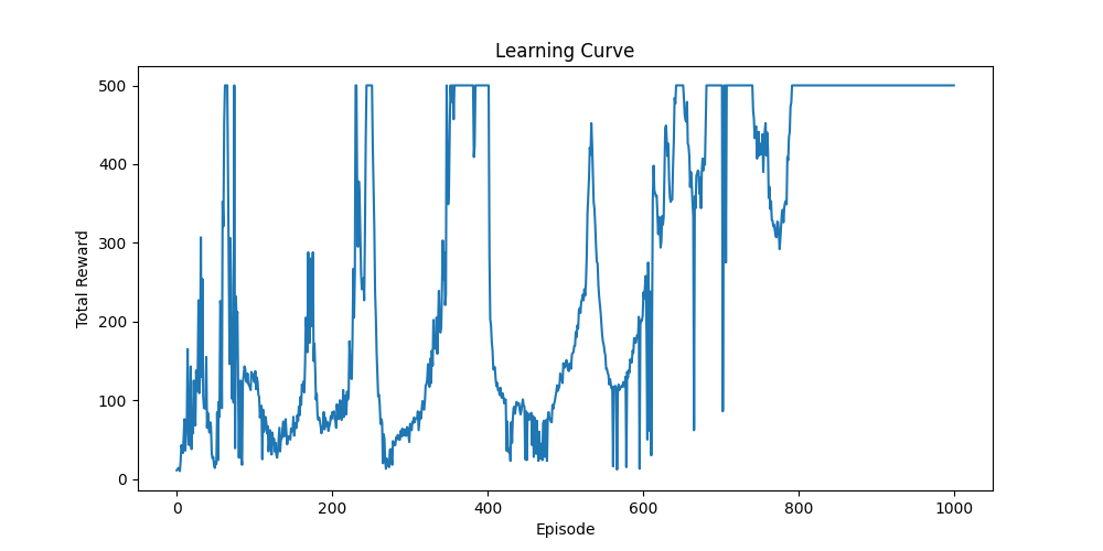
However, a decrease in reward often occurs when the policy becomes too deterministic—repeating the same actions without sufficient exploration—or when the learning updates are too aggressive, causing the policy to overshoot optimal behavior. This is similar to how a person, after initial success, might become rigid in their approach, failing to adapt to new situations or explore better strategies. To address these issues, we will explore more robust methods such as TRPO, PPO, and GPO, which are designed to improve stability and maintain a balance between exploration and exploitation.

Finally, the playing of the trained model looks like this:

Conclusion

In this post, we explored REINFORCE, one of the earliest policy gradient methods, and examined its ability to handle tasks with discrete action spaces. Although REINFORCE is rarely used in practical applications today due to its high variance and lack of stability, it remains a cornerstone in the development of modern policy gradient algorithms. Studying REINFORCE provides valuable insight into the foundations of RL, and its core principles continue to influence ongoing research in more advanced methods such as PPO and TRPO.