Temporal Difference

We talked about Monte Carlo in RL its usage. However, the MC method is not well-suited for online learning, especially in tasks such as autonomous driving, where decisions need to be made continuously and in real-time. This is where the TD method becomes more appropriate, as it allows learning to occur incrementally after each step, making it better suited for online scenarios.
Temporal Difference Introduction
The TD method in RL combines key ideas from both DP and the Monte Carlo method to learn how to predict future rewards and make decisions within an environment. Like the Monte Carlo method, TD is a model-free approach, meaning it does not require a model of the environment’s dynamics.
The TD method updates value estimates based on the TD error, which is the difference between the current value prediction and a new estimate. This new estimate incorporates the reward just received and the predicted value of the next state. The TD error is defined as follows:
$$V_{t+1}(s) \leftarrow V_t(s) + ⍺(R_{t+1} + γV_t(S_{t+1}) - V_t(S_t))1(S_t=s)$$
$$\delta_{t+1} = R_{t+1} + γV_t(S_{t+1}) - V_t(S_t)$$
$$V_{t+1}(s) \leftarrow V_t(s) + ⍺\delta_{t+1}1(S_t=s)$$
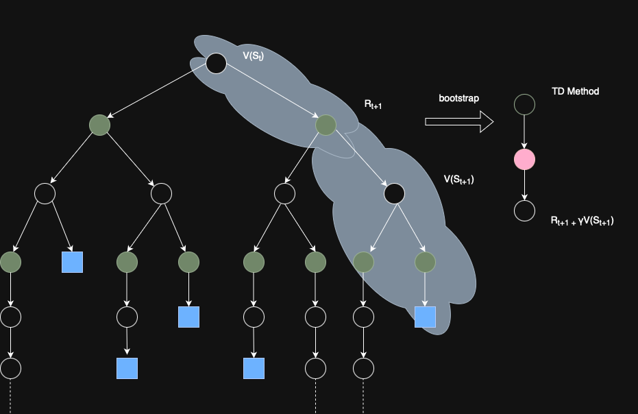
It is easier to understand the TD method by looking at a diagram. From the diagram, we can observe that the TD method estimates the value of a state by looking only one step ahead, using the immediate reward and the value of the next state. This is known as one-step TD.
While one-step TD is simple and efficient, it comes with trade-offs: it tends to have high bias but low variance compared to Monte Carlo methods, which look all the way to the end of an episode.
$$G_{t}^{(n)} = R_{t+1} + γR_{t+2} + γ^2R_{t+3} + \cdots + γ^{n-1}R_{t+n} + γ^nV_{t}(S_{t+n})$$
As you can see, if n=T−t, where T is the end of the episode, the n-step TD return becomes equivalent to the Monte Carlo return. In other words, Monte Carlo can be seen as a special case of n-step TD where the return is calculated using the entire episode.
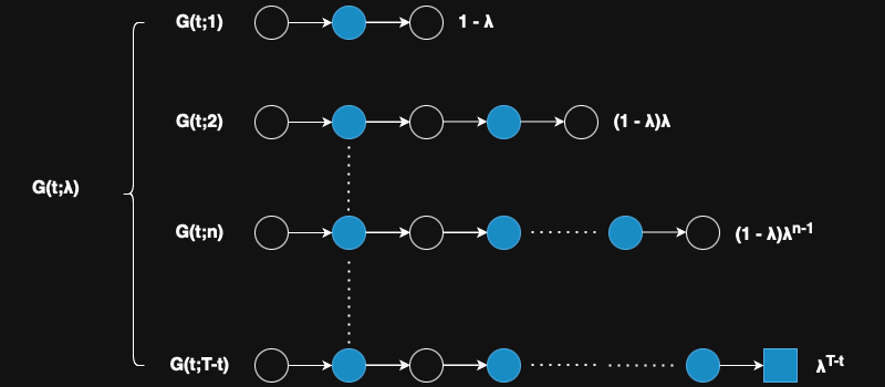
$$G_t^{λ}=(1 - λ)\sum_{n=1}^{T-t} λ^{n-1} G_{t}^{(n)} + λ^{T-t}G_t$$
- TD method: $λ = 0$
- MC method: $λ = 1$
Based on the λ return definition, we can write the value function this way.
$$V_{t+1}(s) = V_t(s) + ⍺(G_{t}^λ - V_t(S_t))1(S_t=s)$$
TD Implementation
To better understand how TD methods differ from MC methods, it is helpful to use the same example we used previously for MC method. However, in this case, we assume a slightly different reward structure: instead of receiving a single reward only upon reaching the terminal state, we now receive a reward after every action taken.
This ongoing feedback allows TD methods to update value estimates incrementally at each step, rather than waiting until the end of an episode as in the MC approach.
import numpy as np
import matplotlib.pyplot as plt
import seaborn as sns
from collections import defaultdict

class BlackjackTD:
    def __init__(self, alpha=0.1, gamma=1.0):
        self.deck = self._create_deck()
        self.action_values = defaultdict(lambda: {'hit': 0, 'stand': 0})
        self.action_counts = defaultdict(lambda: {'hit': 0, 'stand': 0})
        self.episode_rewards = []
        self.alpha = alpha  # Learning rate
        self.gamma = gamma  # Discount factor

    def _create_deck(self):
        """Create a deck of cards (1-10, with face cards as 10)"""
        return list(range(1, 11)) * 4  # 4 suits

    def _draw_card(self):
        """Draw a random card from the deck"""
        return np.random.choice(self.deck)

    def _get_hand_value(self, hand):
        """Calculate the value of a hand, handling aces (1 or 11)"""
        value = sum(hand)
        if 1 in hand and value + 10 <= 21:
            value += 10
        return value

    def _is_bust(self, hand):
        """Check if a hand is bust (over 21)"""
        return self._get_hand_value(hand) > 21

    def _dealer_play(self, dealer_hand):
        """Dealer plays according to standard rules (hit on 16 or less)"""
        while self._get_hand_value(dealer_hand) < 17:
            dealer_hand.append(self._draw_card())
        return dealer_hand

    def _get_state(self, player_hand, dealer_card):
        """Get the current state of the game"""
        return (self._get_hand_value(player_hand), dealer_card)

    def _get_action_value(self, state, action):
        """Get the current value estimate for a state-action pair"""
        return self.action_values[state][action] \
          / max(1, self.action_counts[state][action])

    def _choose_action(self, state, epsilon=0.1):
        """Choose action using epsilon-greedy policy"""
        if np.random.random() < epsilon:
            return np.random.choice(['hit', 'stand'])

        hit_value = self._get_action_value(state, 'hit')
        stand_value = self._get_action_value(state, 'stand')
        return 'hit' if hit_value > stand_value else 'stand'

    def play_episode(self):
        """Play one episode of blackjack using TD(0) learning"""
        player_hand = [self._draw_card(), self._draw_card()]
        dealer_hand = [self._draw_card(), self._draw_card()]
        dealer_card = dealer_hand[0]

        current_state = self._get_state(player_hand, dealer_card)
        episode_reward = 0

        while True:
            # Choose action using epsilon-greedy policy
            action = self._choose_action(current_state)
            self.action_counts[current_state][action] += 1

            # Take action and observe next state and reward
            if action == 'hit':
                player_hand.append(self._draw_card())
                if self._is_bust(player_hand):
                    reward = -1
                    next_state = None  # Terminal state
                else:
                    reward = 0
                    next_state = self._get_state(player_hand, dealer_card)
            else:
                dealer_hand = self._dealer_play(dealer_hand)
                dealer_value = self._get_hand_value(dealer_hand)
                player_value = self._get_hand_value(player_hand)

                if self._is_bust(dealer_hand):
                    reward = 1
                elif dealer_value > player_value:
                    reward = -1
                elif dealer_value < player_value:
                    reward = 1
                else:
                    reward = 0
                next_state = None

            current_value = self._get_action_value(current_state, action)
            if next_state is None:
                next_value = 0
            else:
                # Choose best action for next state
                next_action = self._choose_action(next_state, epsilon=0)
                next_value = \
                  self._get_action_value(next_state, next_action)

            # Update value estimate
            td_target = reward + self.gamma * next_value
            td_error = td_target - current_value
            self.action_values[current_state][action] += \
              self.alpha * td_error

            episode_reward += reward

            if next_state is None:
                break

            current_state = next_state

        self.episode_rewards.append(episode_reward)

    def get_policy(self):
        """Get the current policy (best action for each state)"""
        policy = {}
        for state in self.action_values:
            hit_value = self._get_action_value(state, 'hit')
            stand_value = self._get_action_value(state, 'stand')
            policy[state] = \
              'hit' if hit_value > stand_value \else 'stand'
        return policy

    def plot_learning_curve(self):
        """Plot the learning curve (average reward over time)"""
        plt.figure(figsize=(10, 5))
        window_size = 100
        moving_avg = np.convolve(self.episode_rewards,
                                np.ones(window_size)/window_size,
                                mode='valid')

        plt.plot(moving_avg)
        plt.title('Learning Curve (Moving Average of Rewards)')
        plt.xlabel('Episode')
        plt.ylabel('Average Reward')
        plt.grid(True)
        plt.show()

    def plot_value_function(self):
        """Plot the value function as a heatmap"""
        max_player = 21
        max_dealer = 10
        hit_values = np.zeros((max_player + 1, max_dealer + 1))
        stand_values = np.zeros((max_player + 1, max_dealer + 1))

        for state in self.action_values:
            player_val, dealer_val = state
            if player_val <= max_player and dealer_val <= max_dealer:
                hit_values[player_val, dealer_val] \
                  = self._get_action_value(state, 'hit')
                stand_values[player_val, dealer_val] \
                  = self._get_action_value(state, 'stand')

        plt.figure(figsize=(12, 5))
        plt.subplot(1, 2, 1)
        sns.heatmap(hit_values, cmap='RdYlGn', center=0)
        plt.title('Value Function for Hit')
        plt.xlabel('Dealer Card')
        plt.ylabel('Player Sum')

        plt.subplot(1, 2, 2)
        sns.heatmap(stand_values, cmap='RdYlGn', center=0)
        plt.title('Value Function for Stand')
        plt.xlabel('Dealer Card')
        plt.ylabel('Player Sum')

        plt.tight_layout()
        plt.show()

    def plot_policy(self):
        """Plot the learned policy"""
        policy = self.get_policy()
        max_player = 21
        max_dealer = 10
        policy_matrix = np.zeros((max_player + 1, max_dealer + 1))

        for state, action in policy.items():
            player_val, dealer_val = state
            if player_val <= max_player and \
              dealer_val <= max_dealer:
              policy_matrix[player_val, dealer_val] \
                = 1 if action == 'hit' else 0

        plt.figure(figsize=(8, 8))
        sns.heatmap(policy_matrix, cmap='RdYlGn', center=0.5)
        plt.title('Learned Policy (1=Hit, 0=Stand)')
        plt.xlabel('Dealer Card')
        plt.ylabel('Player Sum')
        plt.show()

def main():
    n_episodes = 10000
    agent = BlackjackTD(alpha=0.1, gamma=0.99)

    print("Training the agent...")
    for i in range(n_episodes):
        agent.play_episode()
        if (i + 1) % 1000 == 0:
            print(f"Completed {i + 1} episodes")

    policy = agent.get_policy()
    print("\nLearned Policy "
          "(Player's Hand Value, Dealer's Card) -> Action:")
    for state, action in sorted(policy.items()):
        print(f"State {state[0]}, {state[1]}: {action}")

    print("\nGenerating plots...")
    agent.plot_learning_curve()
    agent.plot_value_function()
    agent.plot_policy()

if __name__ == "__main__":
    main()
TD(0) - CSY
Also, we can draw the similar heap map like we did in MC method as followed:
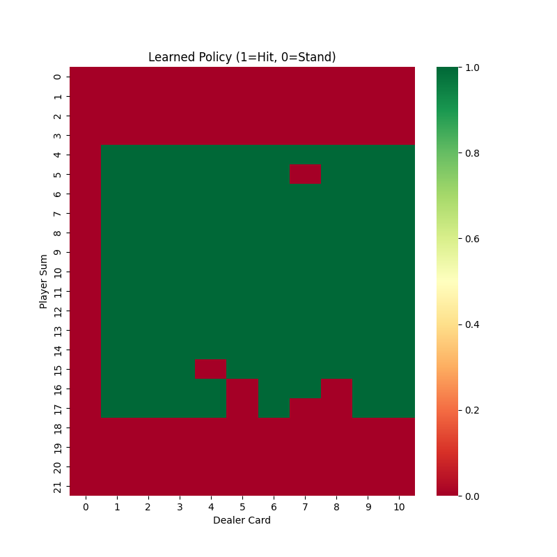
Clearly, the TD method produces better results under the same parameters. This demonstrates that TD typically converges much faster than the MC method, as it updates estimates at every step rather than waiting until the end of an episode. However, there is no one-size-fits-all algorithm—TD methods also have their limitations, such as potential bias due to bootstrapping.
Ultimately, choosing between TD and MC methods (or blending them with TD(λ)) depends on the specific problem, environment characteristics, and what kind of trade-offs the practitioner is willing to accept. Understanding the strengths and weaknesses of each approach is essential for making the right choice.
Conclusion
TD methods, including TD(0) and TD(λ), are foundational in RL, offering a powerful, model-free approach to learning value functions or policies from experience. By updating predictions based on the TD error, they balance the immediate feedback of dynamic programming and the long-term perspective of Monte Carlo methods.
TD(0) is simple and effective for single-step updates, while TD(λ) generalizes this by incorporating multi-step updates via eligibility traces which we will talk in another post, improving efficiency and flexibility.
When paired with deep neural networks, TD methods use the squared TD error as an objective function, enabling scalable learning in complex tasks. Despite challenges like sensitivity to hyperparameters and potential instability with function approximation, TD methods remain versatile and widely used due to their incremental learning, adaptability to non-episodic tasks, and ability to handle sequential decision-making problems effectively.


