Value/Policy-Based Control

Before diving into corporate reinforcement learning with deep neural networks, it's important to understand two fundamental concepts: the difference between policy-based and value-based approaches, and the distinction between on-policy and off-policy methods.
Value-Based v.s. Policy-Based
What are the difference between these two? Let's check their definition first.
- Value-Based: learn a value function which estimates being in a state when following a certain policy. The policy is derived indirectly by selecting actions that maximize the value function.
- E.g., Q-Learning, SARSA
- Policy-Based: learn a policy, which is a mapping (𝑓: X → Y) from state to actions to dictates what action the agent should take in a given state.
- E.g., REINFORCE, Proximal Policy Optimization (PPO)
The definitions and examples of these concepts are clear, but when I first encountered the terms, I found them confusing—it wasn’t easy to imagine how they applied to real-world problems. If I were to generalize, I’d say value-based methods are like strategists, while policy-based methods are more like improvisers. To truly grasp the difference between them, it's helpful to visualize their behaviors in a familiar setting—such as the classic grid world task.
import numpy as np
import matplotlib.pyplot as plt
from typing import Tuple, List
import random

class GridWorld:
    def __init__(self, size: int = 3):
        self.size = size
        self.state = 0  # Start at top-left
        self.goal = size * size - 1  # Goal at bottom-right
        self.actions = [0, 1, 2, 3]  # Up, Right, Down, Left

    def reset(self) -> int:
        self.state = 0
        return self.state

    def step(self, action: int) -> Tuple[int, float, bool]:
        row = self.state // self.size
        col = self.state % self.size

        if action == 0:  # Up
            row = max(0, row - 1)
        elif action == 1:  # Right
            col = min(self.size - 1, col + 1)
        elif action == 2:  # Downj
            row = min(self.size - 1, row + 1)
        elif action == 3:  # Left
            col = max(0, col - 1)

        self.state = row * self.size + col

        # Reward: -1 for each step, +10 for reaching goal
        reward = -1
        done = self.state == self.goal
        if done:
            reward = 10

        return self.state, reward, done

class QLearning:
    def __init__(self,
      n_states: int, n_actions: int,
      learning_rate: float = 0.1, gamma: float = 0.99,
      epsilon: float = 0.1):
        self.q_table = np.zeros((n_states, n_actions))
        self.lr = learning_rate
        self.gamma = gamma
        self.epsilon = epsilon

    def choose_action(self, state: int) -> int:
        if random.random() < self.epsilon:
            return random.choice([0, 1, 2, 3])
        return np.argmax(self.q_table[state])

    def learn(self, state: int, action: int,
              reward: float, next_state: int):
        old_value = self.q_table[state, action]
        next_max = np.max(self.q_table[next_state])
        new_value = (1 - self.lr) * old_value \
          + self.lr * (reward + self.gamma * next_max)
        self.q_table[state, action] = new_value

class REINFORCE:
    def __init__(self, n_states: int,
        n_actions: int, learning_rate: float = 0.01,
        gamma: float = 0.99):
        # Initialize with uniform distribution
        self.policy = np.ones((n_states, n_actions)) / n_actions
        self.lr = learning_rate
        self.gamma = gamma

    def choose_action(self, state: int) -> int:
        probs = self.policy[state]
        probs = np.maximum(probs, 0)
        probs = probs / np.sum(probs)
        return np.random.choice(len(probs), p=probs)

    def learn(self, states: List[int],
      actions: List[int],
      rewards: List[float]):
        returns = []
        G = 0
        for r in reversed(rewards):
            G = r + self.gamma * G
            returns.insert(0, G)

        returns = np.array(returns)
        returns = (returns - returns.mean()) \
          / (returns.std() + 1e-8)  # Normalize returns

        for state, action, G in zip(states, actions, returns):
            self.policy[state] += self.lr * G * (np.eye(len(self.policy[state]))[action] - self.policy[state])
            self.policy[state] = np.maximum(self.policy[state], 0)
            self.policy[state] = self.policy[state] \
              / np.sum(self.policy[state])

def train_and_plot():

    env = GridWorld()

    n_episodes = 1000
    n_states = env.size * env.size
    n_actions = len(env.actions)

    q_agent = QLearning(n_states, n_actions)
    q_rewards = []
    reinforce_agent = REINFORCE(n_states, n_actions)
    reinforce_rewards = []


    # Train Q-learning
    for _ in range(n_episodes):
        state = env.reset()
        total_reward = 0
        done = False

        while not done:
            action = q_agent.choose_action(state)
            next_state, reward, done = env.step(action)
            q_agent.learn(state, action, reward, next_state)
            state = next_state
            total_reward += reward

        q_rewards.append(total_reward)

    # Train REINFORCE
    for _ in range(n_episodes):
        state = env.reset()
        states, actions, rewards = [], [], []
        done = False

        while not done:
            action = reinforce_agent.choose_action(state)
            next_state, reward, done = env.step(action)

            states.append(state)
            actions.append(action)
            rewards.append(reward)

            state = next_state

        reinforce_agent.learn(states, actions, rewards)
        reinforce_rewards.append(sum(rewards))

    # Plot results
    plt.figure(figsize=(12, 5))

    # Calculate average rewards over 10-episode intervals
    def calculate_average_rewards(rewards, interval=10):
        return [np.mean(rewards[i:i+interval]) \
          for i in range(0, len(rewards), interval)]

    q_avg_rewards = calculate_average_rewards(q_rewards)
    reinforce_avg_rewards = calculate_average_rewards(reinforce_rewards)

    episodes = np.arange(0, n_episodes, 10)

    plt.subplot(1, 2, 1)
    plt.plot(episodes, q_avg_rewards, label='Q-learning')
    plt.title('Q-learning Average Rewards (10-episode intervals)')
    plt.xlabel('Episode')
    plt.ylabel('Average Reward')
    plt.legend()

    plt.subplot(1, 2, 2)
    plt.plot(episodes, reinforce_avg_rewards, label='REINFORCE')
    plt.title('REINFORCE Average Rewards (10-episode intervals)')
    plt.xlabel('Episode')
    plt.ylabel('Average Reward')
    plt.legend()

    plt.tight_layout()
    plt.show()

    # Visualize learned policies
    def visualize_policy(policy, title):
        grid = np.zeros((env.size, env.size))
        arrows = ['↑', '→', '↓', '←']

        for state in range(n_states):
            row = state // env.size
            col = state % env.size
            action = np.argmax(policy[state])
            grid[row, col] = action

        plt.figure(figsize=(6, 6))
        plt.imshow(grid, cmap='viridis')
        plt.title(title)

        for i in range(env.size):
            for j in range(env.size):
                state = i * env.size + j
                action = np.argmax(policy[state])
                plt.text(j, i, arrows[action],
                  ha='center', va='center', color='white')

        plt.axis('off')
        plt.show()

    visualize_policy(q_agent.q_table, 'Q-learning Policy')
    visualize_policy(reinforce_agent.policy, 'REINFORCE Policy')

if __name__ == "__main__":
    train_and_plot()
Value/Policy-Based Comparison - CSY
The code above illustrates how value-based and policy-based methods work, respectively. In particular, you can see the key difference in how they initialize and represent knowledge: value-based methods use a Q-table to store action values, whereas policy-based methods rely on a probability distribution (a uniform distribution, in this case) to guide the agent’s behavior. Let's take a look at the diagrams to visualize this difference more clearly.
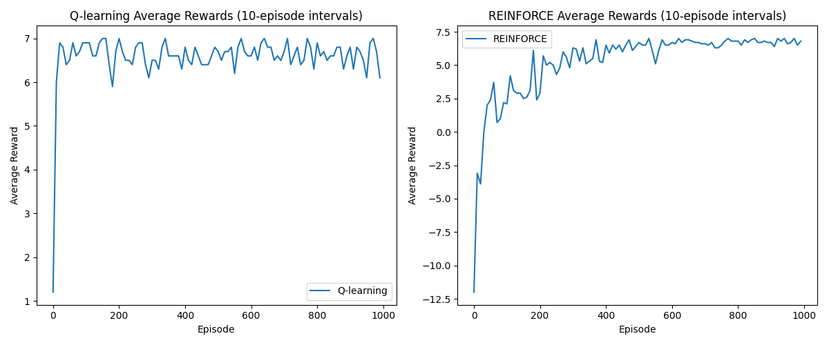
Obviously, both approaches perform well in this grid-world task. However, we observe that the value-based method converges faster than the policy-based one. This is because the value-based approach leverages immediate feedback and doesn't require sampling entire trajectories. On the other hand, the policy-based method (e.g., REINFORCE) adjusts action probabilities directly, which allows for more flexible exploration of diverse paths. This characteristic makes it naturally more compatible with deep neural networks. Finally, the learned policies guide the agent as follows:
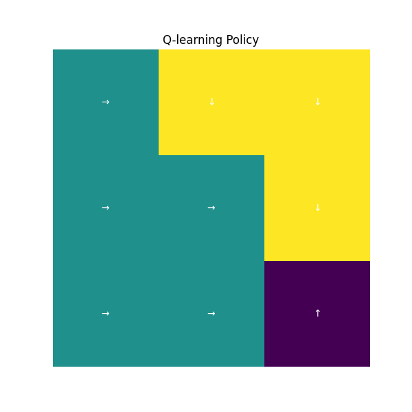
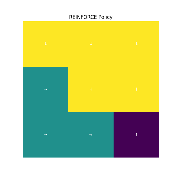
Value-Based(Q-Learning) and Policy-Based (REINFORCE) learned policies - CSY
Conclusion
In RL, value-based and policy-based methods offer distinct approaches to solving problems like navigating a 3x3 grid maze. Policy-based methods (e.g., REINFORCE, TRPO, PPO, GPO) directly learn a probabilistic policy, enabling flexible, exploratory behavior ideal for continuous action spaces or stochastic environments, but they can be sample-inefficient due to high variance.
Value-based methods (e.g., Q-Learning, DQN, Dyna-Q) learn a value function to select actions that maximize expected rewards, offering sample efficiency and stability in discrete action spaces, but they rely on explicit exploration and struggle with continuous actions.
Hybrid methods like actor-critic combine their strengths for robust performance. Choose policy-based for flexibility, value-based for efficiency, or hybrids for complex task.
"What I cannot create, I do not understand." — Richard P. Feynman


