Vanilla Actor-Critic (VAC)

We have previously discussed the Actor Critic and Soft Actor Critic (SAC) frameworks. Today, I would like to revisit its most fundamental form in order to build a deeper understanding and connect it to real-world applications. Specifically, I will focus on the Vanilla Actor–Critic (VAC) algorithm, explaining its details step by step, and then demonstrate how it can be applied to a simple stock prediction task.
In brief, actor is the one who takes actions, and critic is the one who evaluates each action.
Formal Definition of Vanilla Actor-Critic
In a Markov Decision Process (MDP), elements are defined by the tuple $(S,A,P,R,\gamma)$, where:
- $S$: Set of states
- $A$: Set of actions
- $P(s'|s,a)$: Transition probability to next state given state and action
- $R$: Reward function
- $\gamma \in [0, 1)$: Discount factor
same as before, the objective function which maximize the expected cumulative discounted reward is defined as:
$$J(\theta) = 𝔼_{π_\theta}[\sum_{t=0}^∞ \gamma^t r_t]$$
- $π_{\theta}$: parameterized policy (controlled by actor network) with θ
- $r_t = R(s_t,a_t,s_{t+1})$
Components
- Actor: represents the policy $π_{\theta}(a|s)$, which maps state $s \in S$ to a probability distribution over actions $a \in A$, usually updated with Policy Gradient Method to increase the likelihood of actions.
- Critic: estimates the state-value function $V_{\phi}(s)$, parameterized by $\phi$, which represetns the expected cumulative reward starting from state $s$ under policy $π_{\theta}$:
$$V_{\phi}(s) \approx 𝔼_{π_{\theta}}[\sum_{t=0}^∞ \gamma^t r_t | s_0 = s]$$
Updates Rules
Here shows the rules simply.
- Policy Gradient (Actor Network)
$$\nabla_{\theta}J(\theta) = 𝔼_{π_{\theta}}[\nabla_{\theta} \log_{π_{\theta}}(a_t|s_t) \cdot A(s_t, a_t)]$$
$$A(s_t,a_t) \approx \delta_t = r_t + \gamma V_{\phi}(s_{t+1} - V_{\phi}(s_t)$$
Notice the advantage function is the basic temporal difference zero (TD-0) form. Once everything is set up, simply update the parameter θ.
$$\theta \leftarrow \theta + \alpha_1 \cdot \nabla_{\theta} \log {π_{\theta}(a_t|s_t)} \cdot \delta_t$$
- Value Function (Critic Network)
Use gradient descent on the square TD-error to approximate the wanted value function under optimal policy $π^{*}$.
$$\delta_t = r_t + \gamma V_{\phi} (s_{t+1}) - V_{\phi}(s_t)$$
$$\phi \leftarrow \phi + \alpha_2 \cdot \delta_t \cdot \nabla_{\phi} V_{\phi}(s_t)$$
Check detail for Policy Gradient Theorem at the following posts.

Real-World Application - Stock Prediction
I implemented stock prediction using the VAC algorithm with a fixed window size of 30 days, trained on two years of data. For this experiment, I selected SOFI and NDVA as the target stock. The dataset contains a total of 502 trading days, which I split into 386 days for training and 97 days for testing.
The feature set I used for training includes:
- Returns
- High–Low Percentage (High_Low_Pct)
- Open–Close Percentage (Open_Close_Pct)
- Relative Strength Index (RSI)
- Bollinger Band Position (BB_Position)
- Volume Ratio
- Price-to-MA5 Ratio
- Price-to-MA10 Ratio
- Price-to-MA20 Ratio
Of course, additional indices or factors can be incorporated if doing so improves both the accuracy and interpretability of the model in capturing trend fluctuations.
The following results illustrate the overall portfolio changes and the corresponding trading actions.
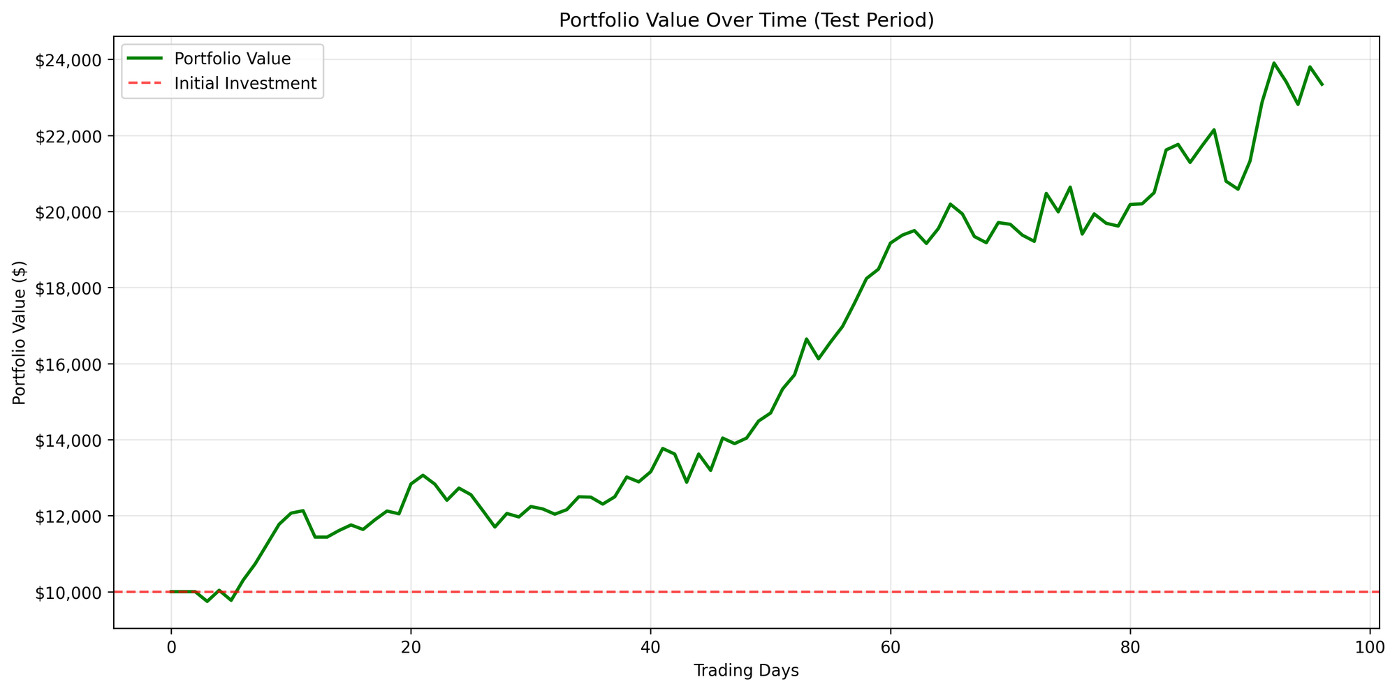
Figure A: SOFI
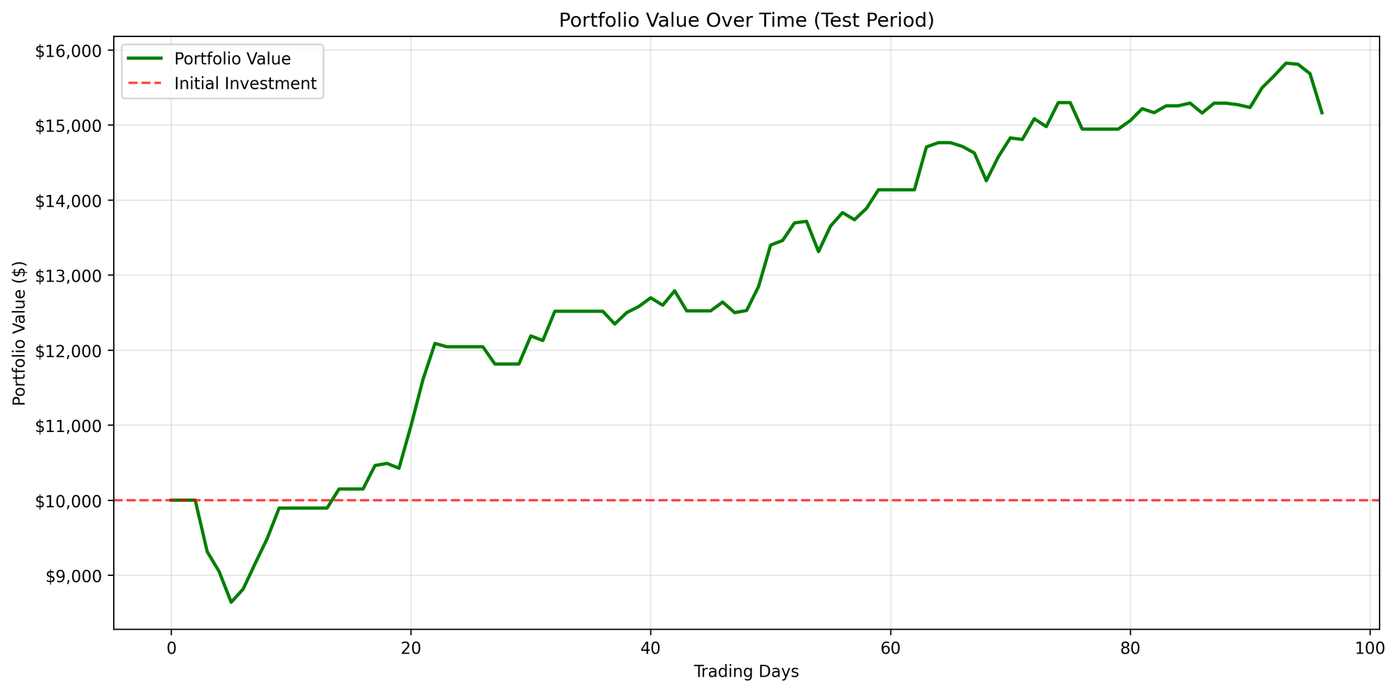
Figure B: NVDA
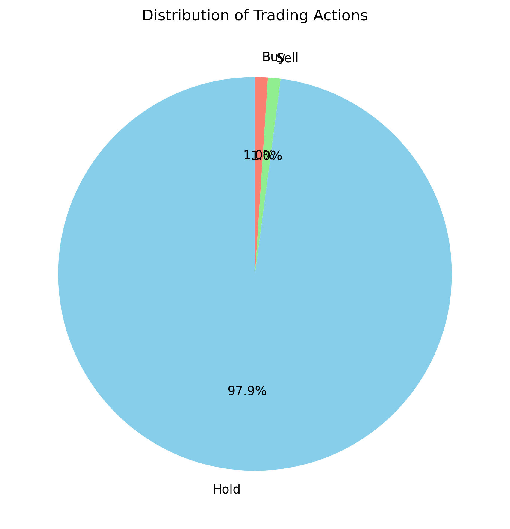
Figure A: SOFI
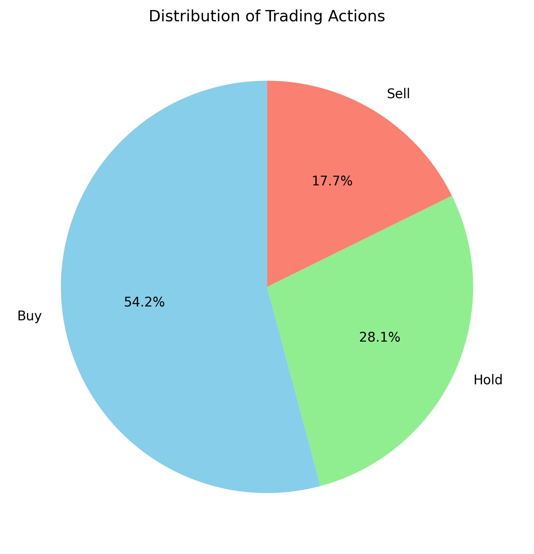
Figure B: NVDA
However, for SOFI, we observe that the majority of actions involve simply holding the position. This is largely a result of its trending behavior, as such a non-stationary environment is inherently difficult to predict. Nevertheless, this implies that for similar stocks, the optimal strategy may often be to hold rather than trade frequently.
In contrast, NVDA exhibits a distinctly different distribution of actions. Understanding the differences between these two cases is crucial for interpreting how the model adapts to varying market dynamics.


